The following chapter provides an example on how to carry out an intersectional analysis of the GEAM data, using the MAIHDA approach, Multilevel Analysis of Individual Heterogeneity and Discriminatory Accuracy.
Keywords
intersectionality, MAIHDA
Although the GEAM questionnaire has been designed for capturing primarily data on gender inequalities, it also offers the opportunity to explore inequalities in relation to other socio-demographic variables. As described in Chapter 2, questions on other important dimensions of discrimination such as sexual orientation, ethnic minority status, or disability / healh impairments among others are included by default in the GEAM questionnaire. The set of socio-demographic variables can then be explored in relation to experiential variables such as experiences of discrimination, microaggressions, job satisfaction, or bullying and harassment.
When examining inequalities across multiple categories, it is important to use an intersectional analytical lens. Intersectionality, as a critical framework, reveals that although we tend to put people into separate boxes according to their socio-demographic features, they are all affected by interlocking processes of discrimination and marginalization (Collins 2015). Intersectionality urges us to see and address the power relations that push women but also many minoritized groups (trans, ethnic minority, non-binary genders, sexual minorities, people with disabitlies) to the margin of society.
While most introductions to intersectionality focus on socio-demographic categories such as gender and race, highlighting how these overlap to produce unique locations of oppression - Black Women (Crenshaw 1990/1991) - this is not enough. Intersectionality is never only about overlapping socio-demographic categories but more importantly about the underlying power dynamics of sexism, racism, ableism that advantage and privilege some while they disenfranchise and marginalize many others:
“Intersectionality is a black feminist theory of power that recognizes how multiple systems of oppression, including racism, patriarchy, capitalism, interact to disseminate disadvantage to and institutionally stratify different groups. Born out of black women’s theorizations of their experiences of racism, sexism, and economic disadvantage from enslavement to Jim Crow to the post-civil rights era, the theory accounts for how systems of oppression reinforce each other, and how their power must be understood not as individually constituted but rather as co-created in concert with each other.” (Robinson 2018, 69)
Intersectionality, insofar it is a theory of power, requires focussing on structures, systems, and institutions that underly and continuously reproduce social inequalities across very different sets of social groups. Each disenfranchised social group is a manifestation of these interlocking systems of stratification and exclusion. Importantly, intersectionality as a critical analytic perspective on power provides an antidote to fractional identity politics. This constitutes the fundamental contribution of Crenshaw: the fight against inequality is not limited to women on the one hand and black men on the other, but happens across these socio-demographic categories, including black women (Crenshaw 1990/1991).
In the context of the GEAM survey, an intersectional analysis provides an entry point for scrutinizing the organisational culture, processes and power relations that marginalize and discriminate some groups while privileging most white men.
6.1 Introduction to MAIHDA
Multilevel Analysis of Individual Heterogeneity and Discriminatory Accuracy (MAIHDA) is a relatively recent approach to carry out an intersectional analysis of quantitative data. It has been pioneered by Clare Evans and others Merlo (2018) to identify intersectional effects, for example with regards to inequalities in health (Axelsson Fisk et al. 2018), mental health (Evans and Erickson 2019), eating disorders (Beccia et al. 2021) or educational outcomes (Keller et al. 2023). Following an intersectional rationale, the MAIHDA analytical framework allows to understand better how the combination of several dimensions of discrimination can have especially aggravating consequences, for example in terms of health.
MAIHDA uses a statistical approach that is known as multilevel modelling. Multilevel models are well established in social sciences to account for the fact that individuals are not isolated atoms but pertain to nested social groupings such as a particular neighbourhood, that is itself part of city which is embedded in a wider region or country. As members of these nested social structures, individuals are exposed to similar living conditions, implied for example when living in a more affluent or more deprived neighbourhood, which affects the quality of life of all residents in a similar degree.
MAIHDA uses the logic of multilevel modelling and conceives individuals (level 1) as members of certain intersectional strata (level 2). Thus, a person might pertain to the stratum of “women + high educational level + minority ethnic group”, while another person pertains to a different stratum, such as “women + low educational level + majority ethnic group”. MAIHDA allows to model how the membership in these intersectional strata affects certain outcomes of interest. This makes it particularly useful for studying inequalities in health, education, and other outcomes such as experiences of discrimination.
Whereas traditional regression models can be used for exploring intersectional effects between several socio-demographic variables such as gender, age, race/ethnicity, they are limited in terms of the number of categories to combine, the sample size, model parsimony and scalability (Evans et al. 2018). In contrast, the MAIHDA approach partitions the variance within and between these strata, and thus can identify unique intersectional effects and provide precise estimates even for small groups.
Described as the new “gold standard” for studying intersectional inequalities (Merlo 2018), several tutorials have been made available that explain the statistical background of MAIHDA Keller et al. (2023). In what follows we adapt the R code provide by Evans, Leckie, et al. (2024) in order to analyse an exemplary GEAM dataset.
An additional tutorial is included in the ggeffects package implementing an intersectional analysis of the EUROFAMCARE data, a study of family cares of older people in Europe.
Small N
While the MAIHDA approach handles small N in each stratum more elegantly than standard regression models, having two few respondents within individual intersectional strata remains an issue.
In the original tutorial Evans, Leckie, et al. (2024) generate 384 intersectional strata combining 2 sex/gender categories x 3 race/ethnicity categories x 4 education categories x 4 income categories x 4 age categories.
The MAIHDA intersectional analysis is only feasible given the dataset contains 33,000 respondents which keeps the grand majority of individual stratum above a minimum of 10 respondents. Keller et al. (2023) in comparison generate 40 intersectional strata for N=5451 students.
GEAM employee data in higher education typically has less than N<1000 respondents, which sets practical limits on the number of intersectional strata to generate. Given we have N=632 respondents in our dataset, we limit the construction of the intersectional data to three variables: gender (women/man), disability/health (yes/no) and age (three age groups), which yields 2x2x3=12 strata. Using MAIHDA we analyse how individuals within these strata are differently affected by experiences of microaggressions. We hypothesize that older age in combination with a disability/health condition and gender (being a women) identifies a group of employees that experience higher microaggressions.
The MAIHDA approach appears as a promising analytical lens especially for GEAM student data which - depending on the size of the higher education institutions - is likely to produce largers samples.
6.2 Preprocess data
First, socio-demographic variables need to be preprocessed as described in Chapter 2. In a second step, the categories of the selected socio-demographic variables are combined to form the intersectional strata.
To start, we remove partial questionnaires. Those respondents who did not reach the end of the survey and press the submit-button have a NA entry in the submitdate and can be removed.
Click to see preprocessing code removing partial submissions
# check how many partial submissions df.geam03 |>group_by(submitdate) |>summarise(Total =n()) |>mutate(Complete =c("Yes", "No"))# remove partial submissionsdf.geam <- df.geam03 |>filter(!is.na(submitdate))
submitdate
Total
Complete
1980-01-01
635
Yes
NA
272
No
Table 6.1: Overview partial and completed questionnaire submissions
Next, gender will be converted to a binary variable. Given that there is only 1 “Non-binary” answer (see Table 6.2) which is not sufficient for defining a distinct stratum, we remove “Non-binary” together with 17 “Prefer not to say” answers from the dataset for variable SDEM004
Click to see code for frequency table
df.geam |>table_frq(SDEM004)
SDEM004
N
Raw%
Valid%
Cum%
A man
175
0.28
0.28
0.28
Non-binary
1
0.00
0.00
0.28
A woman
442
0.70
0.70
0.97
Prefer not to say
17
0.03
0.03
1.00
Table 6.2: Frequency table of raw SDEM004 - Gender
The new variable is renamed from SDEM004 to gender.
Click to see preprocessing code for SDEM004
# create binary gender variable df.geam <- df.geam |>mutate(SDEM004.bin =if_else((SDEM004 =="Non-binary"| SDEM004 =="Prefer not to say"), NA_character_, SDEM004))# re-convert to factordf.geam$gender <-factor(df.geam$SDEM004.bin)
Second, disability and health impairments (SDEM009) contains 30 respondents that prefer not to answer.
Click to see code for frequency table
df.geam |>table_frq(SDEM009)
SDEM009
N
Raw%
Valid%
Cum%
No
479
0.75
0.77
0.77
Yes
107
0.17
0.17
0.94
Prefer not to say
39
0.06
0.06
1.00
NA
10
0.02
0.00
1.00
Table 6.3: Frequency table of raw SDEM009 - Disability and health impairments
We remove those 30 respondents from the dataset before constructing the intersectional strata.
Click to unfold preprocessing code for SDEM009
# replace prefer not to say with NA df.geam <- df.geam |>mutate(SDEM009.bin =if_else(SDEM009 =="Prefer not to say",NA_character_, SDEM009))# reconvert to factordf.geam$disability <-factor(df.geam$SDEM009.bin, levels=c("No", "Yes"), labels=c("No-Disab", "Yes-Disab") )# show frequency tabledf.geam |>table_frq(disability)
disability
N
Raw%
Valid%
Cum%
No-Disab
479
0.75
0.82
0.82
Yes-Disab
107
0.17
0.18
1.00
NA
49
0.08
0.00
1.00
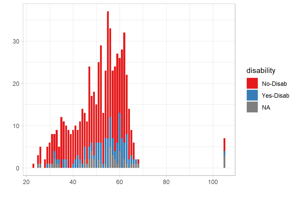
Third, age. Examining the age distribution of the organisation in Figure 6.1, we see that it is left-skewed, meaning that most respondents of the questionnaire are senior employees, with four employees indicating 105 years (to be removed, as this represents an data entry error by respondents). Color coding for disability status, we also see that this overall follows the overall age distribution, having fewer employees that are younger and having a disability compared to more senior employees.
Click to see code for age distribution
# construct three color palettecpal <- RColorBrewer::brewer.pal(3, "Set1")# create barchartdf.geam |>filter(!is.na(age)) |>ggplot(aes(x=age, fill=disability)) +geom_bar(width=0.8) +scale_fill_manual(values=cpal) +labs(x="", y="") +theme_light()
Figure 6.1: Frequency chart of year of birth by disability
Given the senior profiles of most respondents, it is likely that some combinations of strata such as young employees with disabilities will produce too few entries. Hence, we also adjust the thresholds when aggregating the age groups (compared to the procedure described in Section 2.1.2) by shifting the thresholds for junior, middle, and senior profiles slightly up. We create a new variable age_3g consisting of Juniors below 40 years of age, Middle career stage employees from 40 to 54 years of age, and Senior profiles with 55 years or older.
Click to see preprocessing for age groups
#create three age groups: junior, middle, seniordf.geam <- df.geam |>mutate(age_3g =case_when( age <=39~"Junior (<=39)", age >=40& age <55~"Middle (40-54)", age >=55& age <80~"Senior (>=55)",.default =NA ))# reconvert to factordf.geam$age_3g <-factor(df.geam$age_3g)
As can be seen in Table 6.4, the organisation has relatively few junior employees, with most employees in our sample belonging to the senior group, with 45 or more years.
Click to see code for frequency table
df.geam |>table_frq(age_3g)
age_3g
N
Raw%
Valid%
Cum%
Junior (<=39)
102
0.16
0.16
0.16
Middle (40-54)
241
0.38
0.38
0.55
Senior (>=55)
285
0.45
0.45
1.00
NA
7
0.01
0.00
1.00
Table 6.4: Frequency table of 3 age groups
Finally, as outcome variable we use items that form part of the microaggression scale (BIMA001). For each row/respondent, we calculate the average score across all 11 microaggression items (see Section A.4.1 for items) and store the value of each respondent into a new variable called micagg. Higher scores on microagression indicate that respondents have been exposed more frequently to mircoragressions than respondents with lower scores. The following code adjusts the scores to range from “[0]=Never” to “[3]=Often or frequently”; it also removes “[5]=Not applicable” from the mean score calculation by setting it to ‘NA’.
# calculate mean microaggression scores for each respondentdf.tmp <- df.geam |>select(starts_with("BIMA001.SQ"))|>map_df(~ {if_else(.x =="Not applicable", NA, .x)}) |># replace "Not applicable" with NAmap_df(~ {as.numeric(.x) -1}) |># recode scores to 0:3 instead 1:4mutate(micagg =rowMeans(across(everything()), na.rm=T)) |>select(micagg)# incorporate to main data framedf.geam$micagg <- df.tmp$micagg
This provides the following summary statistics in Table 6.5 on our three main socio-demographic variables and the mean score for our outcome variable, namely experiences of microaggressions.
Socio-demographic variables need to be combined to create the intersectional strata for the MAIHDA intersectional analysis. In total, the combination of 2 categories for gender (woman, man), 2 categories for disability (Yes, No) and 3 groups for age generates 2 x 2 x 3 = 12 strata.
Strata
As Evans, Borrell, et al. (2024, 3) describe, strata are descriptors of groups which are theorized as “proxies for the impact of common experiences with social forces” within that group.
Strata are different from social groups, however, as they do not imply social cohesion. Rather, strata capture the social forces such as sexism, racism, classism, abelism that affect individuals pertaining to a particular strata.
Although strata are defined via the combination of socio-demographic variables including sex/gender, ethnicity/race, socioeconomic status, disabilities and others, these cease to be individual-level variables in the MAIHDA analysis and become characteristics describing the social forces acting upon these groups.
The following code creates a unique identifier for each stratum consisting of the combination of labels. NA entries in any of the socio-demographic variables causes the row to be removed.
# generate strata by combining gender, disabilty and age for each row (respondent)# any NA entry of either variable causes the row to be removeddf.geam <- df.geam |>filter(!is.na(gender) &!is.na(disability) &!is.na(age_3g)) |>mutate(strata =paste0(gender, ", ", disability, ", ", age_3g))# convert strata into a factor variabledf.geam$strata <-factor(df.geam$strata)# calculate size of each stratumdf.geam <- df.geam |>group_by(strata) |>mutate(n_strata =n())# calculate percent of strata with less than 10 respondents for 12 subgroupslow <- df.geam |>group_by(strata) |>summarize(n_strata =n()) |>summarize(below_min =sum(n_strata <10)/12) |>pull(below_min)
Each respondent has been assigned the strata which correspondes to the respondents particular combination of gender, disability and age group. Thus 574 respondents (level 1) habe been assigned to 12 strata (level 2). Table 6.6 provides an overview of the number of respondents per strata.
Table 6.6: Frequency table of 11 intersectional strata and number of cases
Given the 12 strata, 2 have fewer than 10 respondents and one stratum has exactly 10 respondents. According Evans, Leckie, et al. (2024) (p.4), a lower bound of 10 respondents per stratum has been deemed acceptable, suggesting that the two strata need to be treated with caution.
For analysis with larger stratum (e.g. > 100) the combination of variable labels becomes impractical. Evans, Leckie, et al. (2024) recommend to geneate a numeric code where each digit represents the levels of variables.
For larger strata, Evans, Leckie, et al. (2024) recommend to calculate the percentage of strata that have less than 10 respondents. For the current example, 17% of our strata have less than 10 respondents.
6.4 MAIHDA Models
Intersectional MAIHDA proceeds in two steps by first, specifing a null model and second a main effects model. The null model characterises the total inequality in our microaggression score between strata. It provides a global measure of intersectionality via the Variance Partition Coefficient (VPC see below), that measures the proportion of the total variance of the outcome that lies between-strata.
The second main effects model allows to quantify how much differences in inequality are due to overlapping axis of inequality. In the statistical model, this implies to partition the outcome/inequality variance into into ‘additive’ (fixed effects) and ‘interaction’ (random effects) part. As described by Evans, Borrell, et al. (2024), the main effects model enables the researcher to “consider inequality patterns in terms of universality-versus-specifity”: are inequalities in outcomes due to universal category membership (e.g. being Black) or by by specific membership in overlapping categories (e.g. being a Black woman). The main effects model specifies to which degree a detected inequality (e.g. wage gap for women) is ‘universal’ across other axis of comparsion (e.g. is true for all women independent of age, race/ethnicity, socioeconomic status, etc.) or differs according to ‘specific’ combinatinos of those variables (e.g. black women having lower wages than white women, etc.). The statistic that describes the relative contribution of additive versus interaction effects is the Proportional Change in Variance (PCV see below).
6.4.1 Model 1: null model
The first step of the MAIHDA approach consists of estimating a null model. It is a simple intersectional model that partitions the variance of the outcome (microaggression score) between and within intersectional strata. At this stage we operate with three different mean values, the sample mean, grand mean, and precision weighted grand mean (see margin).
Sample mean
is simply the mean value across all microagression scores in our sample. In our case, it is 0.41, indicating that most respondents answer either “[0] Never” or “[1] A little or rarely”
Grand mean
calculating the mean value of the microagression score across all strata separately and taking then mean value of the stratum level means yields the grand mean.
Precision weighted grand mean (PWGM)
the PWGM takes the stratum level mean values but weights these according to the size of each stratum. It therefore is a weighted average of the observed stratum means.
# Fit the two-level linear regression with no covariatesmodel_1 <-lmer(micagg ~ (1|strata), data=df.geam)sjPlot::tab_model(model_1,show.reflvl = F,p.style="stars",dv.labels =c("Null Model"))
Null Model
Predictors
Estimates
CI
(Intercept)
0.48 ***
0.36 – 0.59
Random Effects
σ2
0.23
τ00strata
0.03
ICC
0.11
N strata
12
Observations
574
Marginal R2 / Conditional R2
0.000 / 0.113
* p<0.05 ** p<0.01 *** p<0.001
The null model contains only the intercept, which is interpreted as the overall average microaggression score in our dataset. To be more precise, it is the overall precision weighted grand mean (PWGM), which is the mean microaggression score across the mean values of each stratum, weighted by the sample size in each stratum. The PWGM (or intercept) in our example is slightly higher (.48) than the sample mean calculated previously (.41 see Table 6.5).
For further use, we also store the predicted values in the main dataframe.
# store prediced microaggression scores in data framedf.geam$m1Am <-predict(model_1)
Variance Partition Coefficient (VPC)
indicates how important the defined strata are for understanding differences in the outcome of interest, the microaggression score. As such it provides a global notion how important the intersectional strata are for understanding individual inequality.
VPC values range from 0 to 1, where 0 indicates that strata are not important at all, and 1 that strata explain all differences in outcome.
The standard summary model (see above) does not indicate the VPC score of the null model, but we can use the “interclass correlation coefficient (icc)” of the performance package to extract this value. As indicated by Evans, Leckie, et al. (2024), the VPC is identical to the ICC, which indicates how similar the microaggression scores are expected to be between two randomly picked individuals from the same stratum. A high VPC/ICC value (close to 1) indicates that the microaggression scores are expected to be very similar, while a low VPC/ICC score (close to 0) indicates that their microaggression scores are very different between individuals in the same stratum. It thus indicates how strongly the intersectional strata discriminate between groups of individuals that differ with regard to the outcome.
performance::icc(model_1)
ICC_adjusted
ICC_unadjusted
optional
0.1127687
0.1127687
FALSE
VPC values for the null model tend to be <10% (Evans, Borrell, et al. 2024). Keller et al. (2023, 21) in their systematic review report VPC values ranging from 0.5% to 41.9%, with a median value of 5.5%. Similar, Axelsson Fisk et al. (2018) proposes the following cut-off values for VPC/ICC values in percent (%): nonexistent (0–1) - poor (> 1 to ≤ 5) - fair (> 5 to ≤ 10) - good (> 10 to ≤ 20) - very good (> 20 to ≤ 30) - excellent (> 30).
In our example, the ICC value is 0.113, i.e. around 11.3% of the microaggression variance is explained at the stratum level. According to Axelsson Fisk et al. (2018) (see margin), a VPC/ICC score of 11.3% is considered “good”, indicating that a good amount of the variance in the outcome is attributable to between strata level differences. For comparison, Evans, Leckie, et al. (2024) obtain a VPC of 9.4%, qualifying it as “a relatively large amount of clustering at the stratum-level” (p.9).
Hence, our first model and its VPC indicate that strata are important for explaining differences in microaggression scores between intersectional groups. In order to understand the relative importance of individual socio-demographic variables, a second model is however required.
6.4.2 Model 2: main effects model
The main effects model, also called the ‘adjusted intersectional model’ quantifies the extend to which differences between strata level microaggression scores are due to additive (main) effects versus interaction (random) effects.
Thus, we fit a new model (model 1b) adding each socio-demographic variable that defines level-2 strata (gender, disability, age categories) as main additive effects (i.e. as level-2 fixed-effects dummy variables). The variables that define our strata are now incorporated into the model specifically to see how it affects the between strata variance.
The coefficients provide a first orientation on how strong the each socio-demographic variable affect the microaggression score. The larger (in absolute values) the coefficients, the higher the contribution of the variable to the between-stratum variance. In other words, the larger the coefficients, the stronger are the universal effect of a socio-demographic variable that remain relatively uneffected by overlapping axis of inequality.
We see that having a disability / health condition has the strongest effect, as it increments the microaggression score by 27% compared to the reference category (no disability). Gender has a relatively small effect: women tend to have 9% higher microaggression scores compared to the reference category being “A man”. However, this effect is not significant. Age has a comparatively large inverse effect: the older the respondents, the less they are exposed to microaggressions when compared to the reference category “Junior < 35 years”.
Having incorporated the socio-demographic variables into the second model will affect that VPC/ICC score, as it explains now a portion of the variance (of the outcome) directly. The VPC/ICC score will be lower.
performance::icc(model_2)
ICC_adjusted
ICC_unadjusted
optional
0.0697746
0.0659057
FALSE
In the adjusted, main effects model 2, “The VPC now represents the proportion of the total variance that remains (after adjustment for additive effects) that is attributable to interaction effects. By attributable to interaction effects, we mean that some portion of the between-stratum variance (or inequalities) are not adequately described with consistent, additive patterns.” (Evans, Leckie, et al. (2024), p.7)
Model 2, the main effects model, has indeed a much lower VPC value of 6.6%, indicating that the main effects explain a large portion of the between stratum variance, with some stratum inequaity being left unexplained by the additive main effects. To quantify precisely the role of interaction effects, i.e. overlapping axis of inequality, for explaining the variance between strata, we calculate now in addition the Proportional Change in Variance.
Proportional Change in Variance (PCV)
measures how much between-strata variance observed in the intersectional model is explained by additive main effects vs. interaction effects. The complement of this value 1-PCV quantifies how much of the between-stratum variance remains unexplained by the additive main effects and is therefore attributable to interaction affects.
# predict the mean outcome and confidence intervals of predictionm1Bm <-predictInterval(model_2, level=0.95, include.resid.var=FALSE)# predict the stratum random effects and associated SEsm1Bu <-REsim(model_2)
# incorporate predicted values into original data framedf.geam <- df.geam |>bind_cols(m1Bm) |> dplyr::select(gender, disability, age_3g, strata, n_strata, micagg, m1Am,m1Bmfit=fit, m1Bmupr=upr, m1Bmlwr=lwr)# calculate mean for all scoresdf.stratum_level <- df.geam |>group_by(gender, disability, age_3g)|>summarise(across(where(is.numeric), mean), .groups ="drop") |>mutate(rank =rank(m1Bmfit))vc1a <-as.data.frame(VarCorr(model_1))vc1b <-as.data.frame(VarCorr(model_2))# calculate PCVs using components of these variance matrices (as percentages)PCV1 <- ((vc1a[1,4] - vc1b[1,4]) / vc1a[1,4])*100PCV1#> [1] 41.12004
Low PCV values imply that the main effects cannot fully explain the variation in the outcome and that the remaining between-strata variance is due to the existence of interaction effects between the social categories defining the intersectional strata. In contrast, high PCV values indicate that the main additive effects explain a large proportion of the mean-level differences between intersectional strata in the outcome. In our case the PCV indicates that 41.12% of the total variance between strata is accounted for by main additive effects, leaving 58.88% being accounted for by interaction effects.
PCV values usually are rather large. Keller et al. (2023) in reviewing several studies determine a median PCV value of 92.9%, while Evans, Borrell, et al. (2024) indicate typical PCV values to range >80% and frequently >90%. This means that additive effects, i.e. gender, race/ethnicity, disability capture to a large extend inequality patterns across strata. It indicates that inequality patterns are largely additive (in the statistical sense), and less intersectional. In our case, the PCV value is comparatively low, indicating that strong interaction effects between gender, disability and age are at play.
As a summary and to improve readability, model 1 and model 2 can be combined into Table 6.7 which also incorporates the VPC/ICC values and which coefficients are significant.
# only html table.sjPlot::tab_model(model_1, model_2,show.reflvl = F,p.style="stars",dv.labels =c("Null model", "Main effects model"))
Null model
Main effects model
Predictors
Estimates
CI
Estimates
CI
(Intercept)
0.48 ***
0.36 – 0.59
0.44 ***
0.22 – 0.65
gender [A woman]
0.09
-0.09 – 0.28
disability [Yes-Disab]
0.27 **
0.08 – 0.46
age_3gMiddle (40-54)
-0.14
-0.38 – 0.10
age 3g [Senior (>=55)]
-0.18
-0.42 – 0.06
Random Effects
σ2
0.23
0.23
τ00
0.03 strata
0.02 strata
ICC
0.11
0.07
N
12 strata
12 strata
Observations
574
574
Marginal R2 / Conditional R2
0.000 / 0.113
0.055 / 0.121
* p<0.05 ** p<0.01 *** p<0.001
Table 6.7: Parameter estimates for microaggression score, null- and main effects model combined
Disability appears to have a significant effect on the microaggression score. Given the above data, the stratum that comprises women only has on average a microagrression score that is 9% higher than the stratum that only contains men. Similar, strata with individuals that indicate a disability or permanent health condition have a 27% higher microaggression score than strata without a disability. And last but not least, individuals that belong to a senior age group (55 years or older) have on average a 18% lower microaggression score than the reference group (Junior 35 years or younger).
Overall, the model 2 indicates that 41.12% of the between strata variance is explained by these main additive effects of disability and age (and to a lesser degree to gender), with 58.88% of the variance likely being due to interaction effects.
6.5 Visualising & presenting results
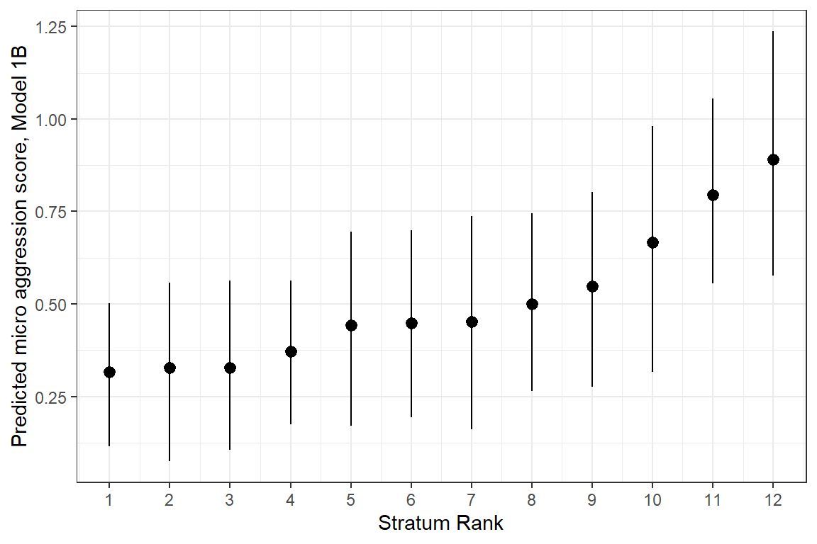
A good way to present MAIHDA results illustrates the predicted microaggression scores for each intersectional strata. Table 6.8 rankes each strata according to the predicted values, placing higher microaggression scores on top and the lowest scores on the bottom.
Table 6.8: Predicted stratum means, order from highest to lowest
As can be seen, the highest microaggression scores are consistenly reported by individuals which indicate a disability or health impairment, across different age groups and genders. A note of caution regarding the strata with small N < 10 - Junior women with disability and Junior men with disabilty. Both have rather high microaggression scores which could change considerably with additional respondents in this age and gender group.
The results of the ranked table can also be illustrated in Figure 6.2.
Our analysis indicates intersectional effects of gender, disability and age for the experience of microaggression. Employees with disabilities in general report higher microaggression scores than employees without. This effect is also stronger for women compared to men. However, small N for two stratum suggest that these estimates could change with higher numbers of respondents (>10). The MAIHA analysis provides in this case a first indication that intersectional effects exist, that warrant further exploration, e.g. with focus groups or interviews with employees with disabilities across different age groups and gender.
Complementing the quantitative analysis with a qualitative exploration is also warranted to understand better how existing power relations and hierarchies within the organisation produce the observed effects.
Further guidance can be found for example in Yang (2023).
References
Axelsson Fisk, Sten, Shai Mulinari, Maria Wemrell, George Leckie, Raquel Perez Vicente, and Juan Merlo. 2018. “Chronic Obstructive Pulmonary Disease in Sweden: An Intersectional Multilevel Analysis of Individual Heterogeneity and Discriminatory Accuracy.”SSM - Population Health 4 (April): 334–46. https://doi.org/10.1016/j.ssmph.2018.03.005.
Beccia, Ariel L., Jonggyu Baek, S. Bryn Austin, William M. Jesdale, and Kate L. Lapane. 2021. “Eating-Related Pathology at the Intersection of Gender Identity and Expression, Sexual Orientation, and Weight Status: An Intersectional Multilevel Analysis of Individual Heterogeneity and Discriminatory Accuracy (MAIHDA) of the Growing Up Today Study Cohorts.”Social Science & Medicine 281 (July): 114092. https://doi.org/10.1016/j.socscimed.2021.114092.
Crenshaw, Kimberle. 1990/1991. “Mapping the Margins: Intersectionality, Identity Politics, and Violence Against Women of Color.”Stanford Law Review 43 (1990/1991): 1241.
Evans, Clare R., Luisa N. Borrell, Andrew Bell, Daniel Holman, S. V. Subramanian, and George Leckie. 2024. “Clarifications on the Intersectional MAIHDA Approach: A Conceptual Guide and Response to Wilkes and Karimi (2024).”Social Science & Medicine 350 (June): 116898. https://doi.org/10.1016/j.socscimed.2024.116898.
Evans, Clare R., and Natasha Erickson. 2019. “Intersectionality and Depression in Adolescence and Early Adulthood: A MAIHDA Analysis of the National Longitudinal Study of Adolescent to Adult Health, 1995–2008.”Social Science & Medicine 220 (January): 1–11. https://doi.org/10.1016/j.socscimed.2018.10.019.
Evans, Clare R., George Leckie, S. V. Subramanian, Andrew Bell, and Juan Merlo. 2024. “A Tutorial for Conducting Intersectional Multilevel Analysis of Individual Heterogeneity and Discriminatory Accuracy (MAIHDA).”SSM - Population Health 26 (June): 101664. https://doi.org/10.1016/j.ssmph.2024.101664.
Evans, Clare R., David R. Williams, Jukka-Pekka Onnela, and S. V. Subramanian. 2018. “A Multilevel Approach to Modeling Health Inequalities at the Intersection of Multiple Social Identities.”Social Science & Medicine 203 (April): 64–73. https://doi.org/10.1016/j.socscimed.2017.11.011.
Keller, Lena, Oliver Lüdtke, Franzis Preckel, and Martin Brunner. 2023. “Educational Inequalities at the Intersection of Multiple Social Categories: An Introduction and Systematic Review of the Multilevel Analysis of Individual Heterogeneity and Discriminatory Accuracy (MAIHDA) Approach.”Educational Psychology Review 35 (1): 31. https://doi.org/10.1007/s10648-023-09733-5.
Merlo, Juan. 2018. “Multilevel Analysis of Individual Heterogeneity and Discriminatory Accuracy (MAIHDA) Within an Intersectional Framework.”Social Science & Medicine 203 (April): 74–80. https://doi.org/10.1016/j.socscimed.2017.12.026.
Robinson, Zandria F. 2018. “Intersectionality and Gender Theory.” In Handbook of the Sociology of Gender, edited by Barbara J. Risman, Carissa M. Froyum, and William J. Scarborough, 69–80. Cham: Springer International Publishing. https://doi.org/10.1007/978-3-319-76333-0_5.
Yang, Keming. 2023. Analysing Intersectionality: A Toolbox of Methods. 1st ed. Thousand Oaks: SAGE Publications.