2  Summarising respondents

Abstract

The following chapter provides an overview of the main socio-demographic variables of the GEAM questionnaire. It briefly introduces each variable and present the most suitable way to describe and visualise the available information.

Keywords

Descriptive statistics, Socio-demographic variables

The GEAM questionnaire gathers various socio-demographic variables from respondents, including gender, age, sexual orientation, ethnic minority status, disability and/or health impairments, educational level, socio-economic class, partnership status, and transgender status. This socio-demographic information forms the basis for identifying differences between specific groups of respondents concerning selected outcomes, such as experiences of discrimination or job satisfaction. Additionally, combinations of these socio-demographic variables enable the exploration of intersectional analyses of GEAM data, revealing how certain combinations of these variables identify particularly disadvantaged sub-groups.

See Chapter 6 for a more detailed example of how to perform an intersectional, outcome oriented analysis of selected GEAM variables.

In addition to socio-demographic variables, the GEAM also contains information on the current job situation of respondents. Variables describe job position, salary, type of contract, scientific discipline among others. These are briefly introduced in section 2 of this chapter. In combination with socio-demographic variables, they provide the basis for detecting wage gaps or differences in precarious working conditions.

In what follows, we briefly introduce each of the available socio-demographic variables and show how to best summarise the available information. Each variable is introduced by describing briefly its answer options. Information on the specific choices of answer options for each variable is availble in Guyan et al. (2022). 

Note

For the following chapter we use two real-world datasets, marked in the code as df.geam01 (Organisation 1) and df.geam02 (Organisation 2) respectively. The main difference between these datasets concerns the way how some variables have been modified and adapted to the specific organisational context. However, this does not affect their interpretability for the descriptive statistics explained in this chapter.

2.1 Socio-demographic variables

As a preparatory step it makes sense to observe the number of partial submissions of the GEAM questionnaire. Partial submissions create many NA entries that can be filtered out before the start of the actual analysis.

A simple way of identifying incomplete questionnaires, consists of looking at the lastpage meta-data field in the questionnaire. An alternative consists of examining the submission date variable submitdate. This field is set to NA if the respondent did not reach the final page and press the submit button of the questionnaire.

df.geam01 |>
  group_by(submitdate) |>
  summarise(Total = n()) |>
  mutate(Complete = c("Yes", "No")) |>
  table_df()

Listing 2.1: Check number of incomplete GEAM submissions

submitdate	Total	Complete
1980-01-01	191	Yes
NA	42	No

In a subsequent step, we can remove incomplete submissions, as shown in Listing 2.2

df.geam <- df.geam01 |>
  filter(!is.na(submitdate))

Listing 2.2: Remove number of incomplete GEAM submissions

2.1.1 Gender

The GEAM includes a standard question about gender identity of the respondent which has four answer options. Compared to other recommended approaches to ask about gender especially in the context of health research (Stadler et al. 2023), this is a relatively simple yet effective approach to capture the most important gender identity options in an organisational context.

Code	Question	Responses
SDEM004	Are you…	[1] A man [2] Non-binary [3] A woman [4] Prefer not to say [5] Prefer to self-identify as:

Responses regarding gender (‘SEM004’) are then easily summarised with a frequency table or bar chart that demonstrates that answer option ‘[2] Non-binary’ or ‘[4] Prefer not to say’ or ’[5] Prefer to self-identify as:” are comparatively few.

As the simple frequency Table 2.1 for ‘SDEM004’ demonstrates, only 2 respondents have selected ‘[4] Prefer not to say’ in this example dataset with answer options ‘[2] Non-binary’ and ‘[5] Other’ having received no responses.

The R code for producing simple frequency tables is using a custom function table_frq() that has been defined in the util/common.R file. You can inspect the contents of this file on the Github repository of this book.

df.geam01 |>
  table_frq(SDEM004)

SDEM004	N	Raw%	Valid%	Cum%
A man	87	0.37	0.40	0.40
A woman	130	0.56	0.59	0.99
Prefer not to say	2	0.01	0.01	1.00
NA	14	0.06	0.00	1.00

Table 2.1: Frequency table of SDEM004 - Gender

Note

In the most recent GEAM version (since v3.0) “Other” as answer-option has been replaced with “Prefer to self-identify as” to avoid othering. As some of our data has been collected with previous GEAM versions, the “Other” label might still be visible in frequency tables and illustrations.

The frequency table can then be transformed into a bar chart, indicating the absolute counts of each gender.

# define colors 
cpal <- RColorBrewer::brewer.pal(4, "Set1")

df.geam01 |> 
    ggplot(aes(x=SDEM004, fill=SDEM004)) + 
    geom_bar(width=.8) + 
    scale_fill_manual(values=cpal, na.value=cpal[4]) +
    guides(fill="none") +
    labs(x="", y="") +
    theme_light()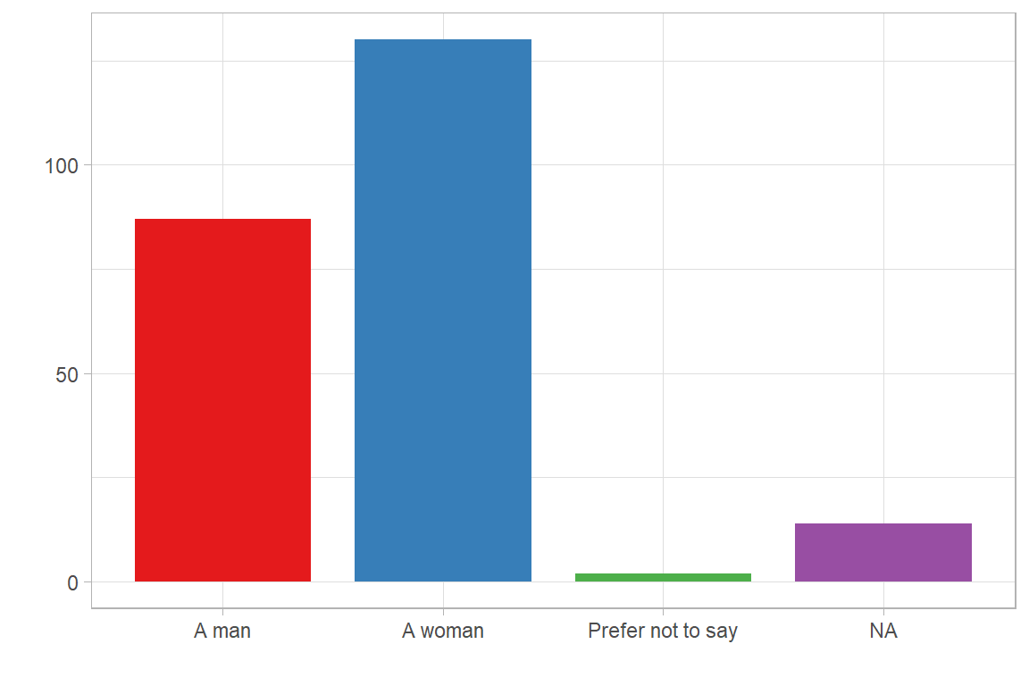

Figure 2.1: Bar chart of SDEM004 - Gender

For further analysis, in some cases a binary gender variable SDEM004.bin needs to be constructed as shown in Listing 2.3 which then can be used for simple cross-tab analysis (see Chapter 3).

df.geam01 <- df.geam01 |>
  mutate(SDEM004.bin = case_when(
    SDEM004 == "Prefer not to say" ~ NA,
    SDEM004 == "Non-binary" ~ NA, 
    SDEM004 == "Other" ~ NA,
    .default = SDEM004
  ))

Listing 2.3: Binarise SDEM004 gender variable

2.1.2 Age

The age of respondents is by captured as an integer variable (SDEM001 - “In which year were you born?”).

df.geam02 |>  
    filter(!is.na(SDEM001)) |>
    ggplot(aes(x=SDEM001)) + 
    geom_bar(width=0.8) + 
    labs(x="", y="") +
    theme_light()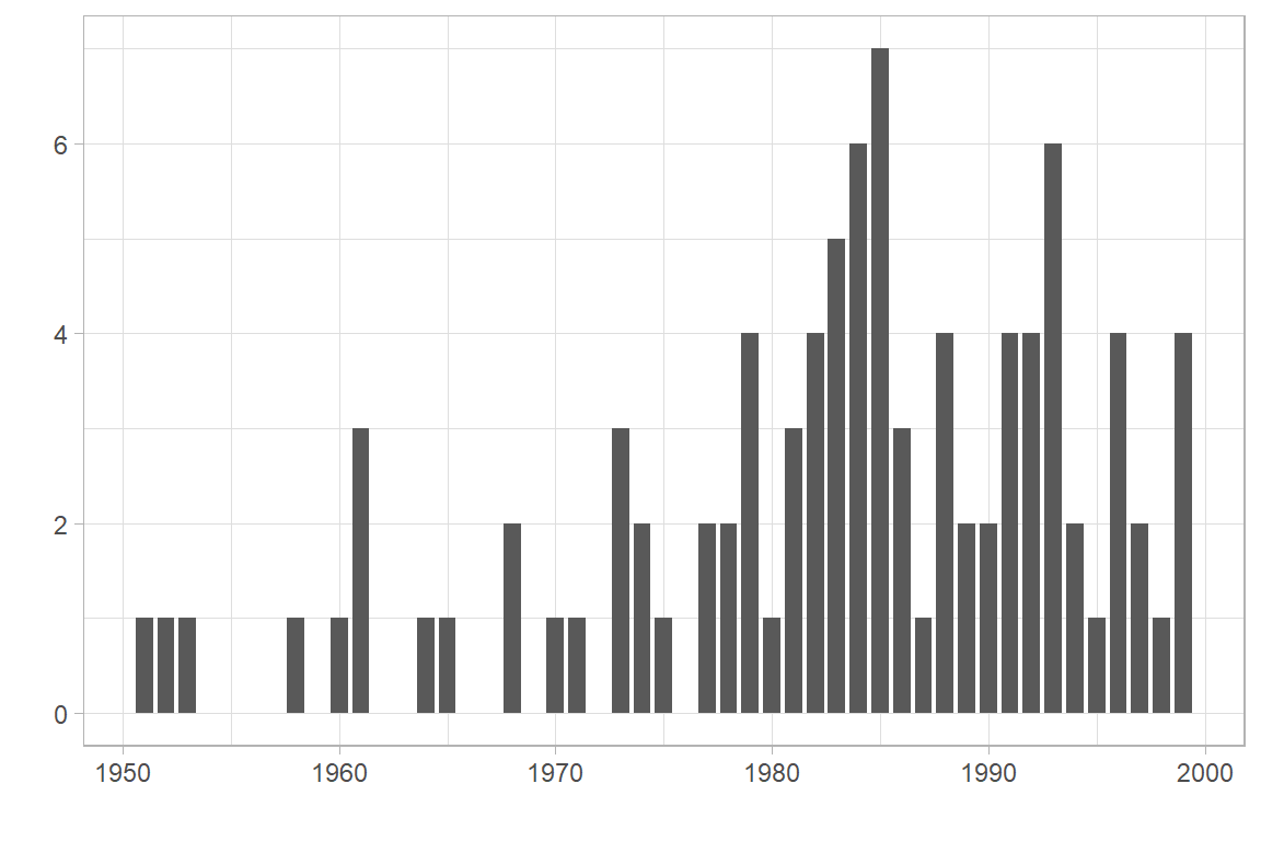

Figure 2.2: Frequency chart of SDEM001 - year of birth

Most statistical analysis will work with aggregated age groups. In R, a small transformation is necessary to convert and aggregated the year of birth into binned age groups. First, the current age is calculated as shown in Listing 2.4

# retrieve current year 
curyear <- as.numeric(format(Sys.Date(), format="%Y"))

# calculate age of respondent for current year
df.geam02$age <- curyear - df.geam02$SDEM001

Listing 2.4: Calculate current age

Listing 2.5 assigns respondents to a specified age group using the newly created age variable with the cut() command. We create four groups.

# sub-divde age into 4 age groups:
df.geam02$age_4g <- cut(df.geam02$age,
                        c(0,29,44,64,100),
                        labels=c("Junior (<=29)", 
                                 "Middle (30-44)", 
                                 "Senior (45-64)", 
                                 "+65"))

Listing 2.5: Aggregate respondents age into 4 age groups

And display the aggregated age groups:

df.geam02 |>  
    ggplot(aes(x=age_4g)) + 
    geom_bar(width=0.8) + 
    labs(x="", y="") +
    theme_light()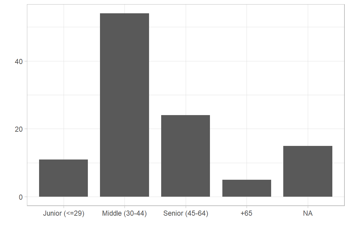

Figure 2.3: Frequency chart of aggregated age groups

Here is the corresponding frequency table:

df.geam02 |>
  table_frq(age_4g) 

age_4g	N	Raw%	Valid%	Cum%
Junior (<=29)	11	0.10	0.12	0.12
Middle (30-44)	54	0.50	0.57	0.69
Senior (45-64)	24	0.22	0.26	0.95
+65	5	0.05	0.05	1.00
NA	15	0.14	0.00	1.00

Table 2.2: Frequency table of aggregated age groups

Other GEAM questionnaires have modified ‘SDEM001’ before the launch and ask for aggregate age groups from the start. This might be advisable to protect respondents anonymity. As a consequence, the aggregation into age groups as explained above is not necessary. Here is an example:

df.geam01 |>  
    filter(!is.na(SDEM001)) |>
    ggplot(aes(x=SDEM001)) + 
    geom_bar(width=0.8) + 
    labs(x="", y="") +
    theme_light()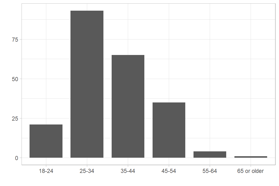

Figure 2.4: Bar chart of SDEM001 - Aggregated age groups

2.1.3 Current marital or partnership status

Question SDEM006 asks about marital or partnership status which becomes especially relevant for inquires with regards to care responsibilities.

Code	Question	Responses
SDEM006	Which best describes your current marital or partnership status?	[1] Single and never married or never in a civil partnership [2] Married or in a civil partnership [3] Cohabiting [4] Separated [5] Divorced [6] Widowed [7] Prefer not to say [8] I prefer to label my current partnership as

df.geam02 |>
  table_frq(SDEM006) 

SDEM006	N	Raw%	Valid%	Cum%
Single and never married or never in a civil partnership	34	0.31	0.36	0.36
Married or in a civil partnership	41	0.38	0.44	0.80
Cohabiting	6	0.06	0.06	0.86
Separated	3	0.03	0.03	0.89
Divorced	10	0.09	0.11	1.00
NA	15	0.14	0.00	1.00

Table 2.3: Frequency table of SDEM006 - Martial and partnership status

cpal <- RColorBrewer::brewer.pal(6, "Set1")

df.geam02 |> 
  ggplot(aes(x=SDEM006, fill=SDEM006)) + 
  geom_bar(width=.8) + 
  scale_fill_manual(values=cpal, na.value=cpal[6]) +
  scale_x_discrete(labels = function(x) str_wrap(x, width = 15)) +
  guides(fill="none") +
  labs(x="", y="") + 
  theme_light()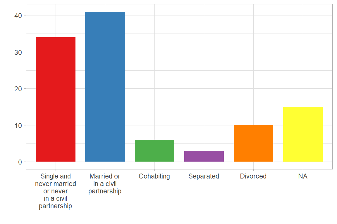

Figure 2.5: Bar chart of SDEM006 - Martial and partnership status

Other variables of interest to be explored in relation to the partnership status concerns the care responsibilities for a dependent adult (WCWI006) or children (WCWI008). Note, that WCWI010 also asks about being a “single parent or legal guardian” for children below the age of 18. Cross-checking SDEM006 with WCWI010 provides a good picture of the potential impact of caring responsibilities of respondents.

2.1.4 Ethnic mayority or minority status

The GEAM inquires about ethnic minority or mayority status in question SDEM002:

Code	Question	Responses
SDEM002	Do you currently perceive yourself to be part of a majority or minority ethnic or racialized group?	[1] Majority [2] Minority [3] Unsure [4] Prefer not to say

As this question is not mandatory, there are likely to be a larger amount of NA entries that need to be removed in subsequent analysis.

df.geam01 |>
  table_frq(SDEM002) 

SDEM002	N	Raw%	Valid%	Cum%
Majority	170	0.73	0.78	0.78
Minority	28	0.12	0.13	0.91
Unsure	11	0.05	0.05	0.96
Prefer not to say	9	0.04	0.04	1.00
NA	15	0.06	0.00	1.00

Table 2.4: Frequency table of SDEM002 - Ethnic minority / majority status

cpal <- RColorBrewer::brewer.pal(5, "Set1")

df.geam01 |> 
  ggplot(aes(x=SDEM002, fill=SDEM002)) + 
  geom_bar(width=.8) + 
  scale_fill_manual(values=cpal, na.value=cpal[5]) +
  guides(fill="none") +
  labs(x="", y="") + 
  theme_light()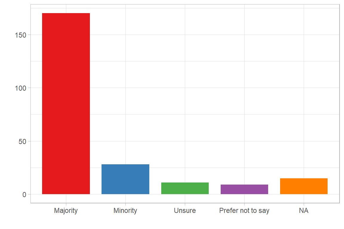

Figure 2.6: Bar chart of SDEM002 - Ethnic minority / majority status

2.1.5 Country of birth and main citizenship

Variable SDEM012 asks about the country of birth of respondents. Again, depending on the privacy concerns when preparing the survey, countries can be aggregated into broader geographic regions in order to protect the anonymity of participants. This is the case in organisation 1 as shown in the following example.

df.geam01 |>
  table_frq(SDEM012) 

SDEM012	N	Raw%	Valid%	Cum%
Eastern Europe	58	0.25	0.27	0.27
Western Europe	65	0.28	0.30	0.57
Southeast Asia	2	0.01	0.01	0.58
South Asia	7	0.03	0.03	0.61
Northern Europe	2	0.01	0.01	0.62
Southern Europe	61	0.26	0.28	0.90
North America	4	0.02	0.02	0.92
Central America	1	0.00	0.00	0.93
Caribbean	1	0.00	0.00	0.93
South America	9	0.04	0.04	0.97
Middle East	2	0.01	0.01	0.98
East Asia	2	0.01	0.01	0.99
Other	2	0.01	0.01	1.00
NA	17	0.07	0.00	1.00

Table 2.5: Frequency table of SDEM012 - Country of birth aggregated into geographic regions. Note the descending order of frequencies produced by sort.frq=‘desc’

Variable SDEM013 inquires about the main citizenship of respondents. Combining both variables SDEM012 and SDEM013 provides insights into possible migration background of respondents, given the specific country context in which the survey is implemented.

2.1.6 Trans history

Question SDEM005 inquires is a respondent “is trans or has a trans history”.

Code	Question	Responses
SDEM005	Are you trans or do you have a trans history	[1] No [2] Yes [3] Prefer not to say

df.geam01 |>
  table_frq(SDEM005) 

SDEM005	N	Raw%	Valid%	Cum%
No	217	0.93	1	1
Yes	1	0.00	0	1
NA	15	0.06	0	1

Table 2.6: Frequency table of SDEM005 - Trans history

2.1.7 Sexual orientation

Variable SDEM007 asks respondents about their sexual orientation - which constitutes another important dimension of social discrimination.

Code	Question	Responses
SDEM007	Which best describes your sexual orientation?	[1] Bisexual [2] Gay / lesbian [3] Heterosexual / straight [4] Prefer not to say [5] Another sexual orientation, please specify:

df.geam01 |>
  table_frq(SDEM007) 

SDEM007	N	Raw%	Valid%	Cum%
Bisexual	18	0.08	0.08	0.08
Gay / lesbian	15	0.06	0.07	0.15
Heterosexual / straight	175	0.75	0.80	0.95
Prefer not to say	8	0.03	0.04	0.99
Other	2	0.01	0.01	1.00
NA	15	0.06	0.00	1.00

Table 2.7: Frequency table of SDEM007 - Sexual orientation. Note that answer option ‘Other’ has been replaced by the latest GEAM version 3 to ‘Another sexual orientation’

Questions that allow respondents to indicate their preferred answer category are marked in the data matrix with the question code (here SDEM007) and the suffix .other. attached. As the Table 2.7 indicates, two respondents indicate an additional option, which can be quickly displayed with the following code:

# Extract text entries from .other. input field
df.geam01 |>
  filter(SDEM007 == "Other") |>
  select(id, SDEM007, SDEM007.other.) 

id	SDEM007	SDEM007.other.
150	Other	pansexual
231	Other	Pansexual

Table 2.8: Extracting ‘other’ response options for SDEM007 - Sexual orienation

Warning

When analysing text input fields one should carefully check the provided information before running any type of analysis as it might contain sensitive information. A respondent might have provided a plain name which should be XXXed-out before proceeding.

2.1.8 Disability and/or health impairments

Variable SDEM009 captures disability and health impairments. This is a fairly generic question that does not inquire about specific medical conditions or impairments. Asking about specific conditions makes sense in case a corresponding diversity or equality policy can address these diverse conditions with specific measures and interventions.

Code	Question	Responses
SDEM009	Do you have any disability, impairments or long term health conditions?	[1] No [2] Yes [3] Prefer not to say

df.geam01 |>
  table_frq(SDEM009) 

SDEM009	N	Raw%	Valid%	Cum%
No	199	0.85	0.91	0.91
Yes	15	0.06	0.07	0.98
Prefer not to say	5	0.02	0.02	1.00
NA	14	0.06	0.00	1.00

Table 2.9: Frequency table of SDEM009 - Disability and health impairments

As can be seen from frequency Table 2.9, among the respondents, 15 persons indicate a disabilty or health impairment.

2.1.9 Educational level

The highest educational level of the respondent is covered in question SDEM016. Responses follow the International Standard Classification of Education (ISCED) proposed by the UNESCO Institute for Statistics (UNESCO Institute for Statistics 2012) which provides the basis for comparing educational levels across countries.

Code	Question	Responses
SDEM016	What is the highest qualification level that you have obtained?	[1] No formal education [2] Primary school / elementary school [3] Secondary school / high school [4] College diploma or degree [5] Technical school [6] University - Baccalaureate / Bacherlor’s [7] University - Master’s [8] University - Doctorate [9] University - Postdoctorate [10] Prefer not to say [11] Other:

df.geam01 |>
  table_frq(SDEM016)

SDEM016	N	Raw%	Valid%	Cum%
Secondary school / high school	2	0.01	0.01	0.01
College diploma or degree	5	0.02	0.02	0.03
Technical school	6	0.03	0.03	0.06
University - Baccalaureate / Bachelor’s	13	0.06	0.06	0.12
University - Master’s	76	0.33	0.35	0.47
University - Doctorate	36	0.15	0.16	0.63
University - Postdoctorate	73	0.31	0.33	0.96
Prefer not to say	2	0.01	0.01	0.97
Other	6	0.03	0.03	1.00
NA	14	0.06	0.00	1.00

Table 2.10: Frequency table of SDEM016 - Highest educational level of respondent

It is likely that some respondents mark “Other” for SDEM016. These need to be examined and re-classified according to the best fit with existing categories. Examining the SDEM016.other. variable we see that 4 out of the 6 respondents have provided an alternative educational category, while 2 respondents have selected the “Other” option but not filled in any alternative text.

# Extract text entries from .other. input field
df.geam01 |>
  filter(SDEM016 == "Other")|>
  select(id, SDEM016, SDEM016.other.) 

id	SDEM016	SDEM016.other.
19	Other	Prof
83	Other	Grado superior FPII
129	Other	NA
192	Other	Diplomatura
224	Other	NA
231	Other	Universidad-Grado

Table 2.11: Extracting ‘other’ response options for SDEM016 - Educational level

The answer questions then can be re-coded as desired (show example).

2.1.10 Socioeconomic status

Educational attainment is among the most widely used indicator for socioeconomic status (SES). Differences in SES have important implications in terms of health- or educational outcomes and thus provide an important indicator of social inequalities (Stadler et al. 2023; APA 2007). Current SES is measured by respondents educational level (SDEM016). In order to track SES of entry level positions in the organisation, including early career researchers, the educational attainment of parents and/or legal guardians should be used.

Socioeconomic status is captured by two variables SDEM017 and SDEM018, one for each parent and/or legal guardian. Note that answer options are indentical to SDEM016 and follow the UNESCO ISCED standard classification.

Code	Question	Responses
SDEM017	What is the highest qualification level obtained by your first parent/guardian?	see responses to SDEM016
SDEM018	What is the highest qualification level obtained by your second parent/guardian?	see responses SDEM016

Frequency table of first parent or legal tutor of respondent.

df.geam01 |>
  table_frq(SDEM017)

SDEM017	N	Raw%	Valid%	Cum%
No formal education	6	0.03	0.03	0.03
Primary school / elementary school	28	0.12	0.13	0.16
Secondary school / high school	35	0.15	0.16	0.32
College diploma or degree	12	0.05	0.06	0.38
Technical school	17	0.07	0.08	0.45
University - Baccalaureate / Bachelor’s	58	0.25	0.27	0.72
University - Master’s	34	0.15	0.16	0.88
University - Doctorate	13	0.06	0.06	0.94
University - Postdoctorate	9	0.04	0.04	0.98
Prefer not to say	3	0.01	0.01	1.00
Other	1	0.00	0.00	1.00
NA	17	0.07	0.00	1.00

Table 2.12: Frequency table of SDEM017 - Highest educational level of parent/legal tutor

And second parent / tutor:

df.geam01 |>
  table_frq(SDEM018)

SDEM018	N	Raw%	Valid%	Cum%
No formal education	9	0.04	0.04	0.04
Primary school / elementary school	29	0.12	0.14	0.18
Secondary school / high school	54	0.23	0.26	0.44
College diploma or degree	12	0.05	0.06	0.50
Technical school	23	0.10	0.11	0.60
University - Baccalaureate / Bachelor’s	43	0.18	0.20	0.81
University - Master’s	32	0.14	0.15	0.96
University - Doctorate	3	0.01	0.01	0.98
University - Postdoctorate	1	0.00	0.00	0.98
Prefer not to say	3	0.01	0.01	1.00
Other	1	0.00	0.00	1.00
NA	23	0.10	0.00	1.00

Table 2.13: Frequency table of SDEM018 - Highest educational level of 1st parent/legal tutor

In preparing the analysis of the SES of respondents, the educational level is ususally aggregated in fewer groups. This involves combining (or selecting) the educational level of parent 1 and 2. For example, one can select the higher educational level comparing parent 1 and 2 and then aggregate this highest educational level of both parents (or legal guardians) into a single variable SES.

To do so, we need some preprocessing of SDEM017 and SDEM018. Listing 2.6 first assigns a new value (-99) to answer options “Prefer not to say”, “Other” and “NA” to make the variables comparable at all.

# create new SES variable based upon the higher value of SDEM017 vs. SDEM018
df.geam01 <- df.geam01 |>
  mutate(SDEM017.comp = if_else(SDEM017 == "Prefer not to say" | 
                                SDEM017 == "Other" | 
                                is.na(SDEM017), -99, as.numeric(SDEM017)), 
         SDEM018.comp = if_else(SDEM018 == "Prefer not to say" |
                                SDEM018 == "Other" | 
                                is.na(SDEM018), -99, as.numeric(SDEM018)), 
         SES = if_else(SDEM017.comp >= SDEM018.comp, SDEM017.comp, SDEM018.comp))

Listing 2.6: Compare SDEM017 and SDEM018 using newly created SES variable

The newly created variable SES now contains the hightest educational level considering both parents. The following code shows the first 6 rows of our dataset, indicating the highest educational level in the last column SES.

df.geam01 |>
  dplyr::select(SDEM017, SDEM017.comp, SDEM018, SDEM018.comp, SES) |>
  head() |>
  table_df()

SDEM017	SDEM017.comp	SDEM018	SDEM018.comp	SES
University - Master’s	7	University - Master’s	7	7
University - Baccalaureate / Bachelor’s	6	University - Baccalaureate / Bachelor’s	6	6
University - Baccalaureate / Bachelor’s	6	Secondary school / high school	3	6
University - Baccalaureate / Bachelor’s	6	University - Baccalaureate / Bachelor’s	6	6
Primary school / elementary school	2	Primary school / elementary school	2	2
University - Master’s	7	Secondary school / high school	3	7

Table 2.14: Comparing highest educational level parent 1 and parent 2

Then it is easy to assign the respondents socioeconomic status to three groups, consisting of “Higher SES”, “Medium SES”, or “Lower SES” as shown in lst-code-ses-3g.

df.geam01 <- df.geam01 |>
  mutate(SES_3g = case_when(
    SES >0 & SES <=3 ~ "Lower SES", 
    SES >3 & SES <=5 ~ "Medium SES",
    SES >5 & SES <=9 ~ "Higher SES",
    .default = NA
  ))

Listing 2.7: Code to aggregate three levels of socio-economic status

A corresponding frequency table or bar chart is then easily created. As shown in Figure 2.7, most respondents have a high socio-economic background given the science and research context of the organisation. Subsequent analysis could further explore how the SES differs between the job positions captured in variable WCJC001 (see next section).

cpal <- RColorBrewer::brewer.pal(3, "Set1")

df.geam01 |> 
  ggplot(aes(x=SES_3g, fill=SES_3g)) + 
  geom_bar(width=.8) + 
  scale_fill_manual(values=cpal, na.value=cpal[6]) +
  guides(fill="none") +
  labs(x="", y="") + 
  theme_light()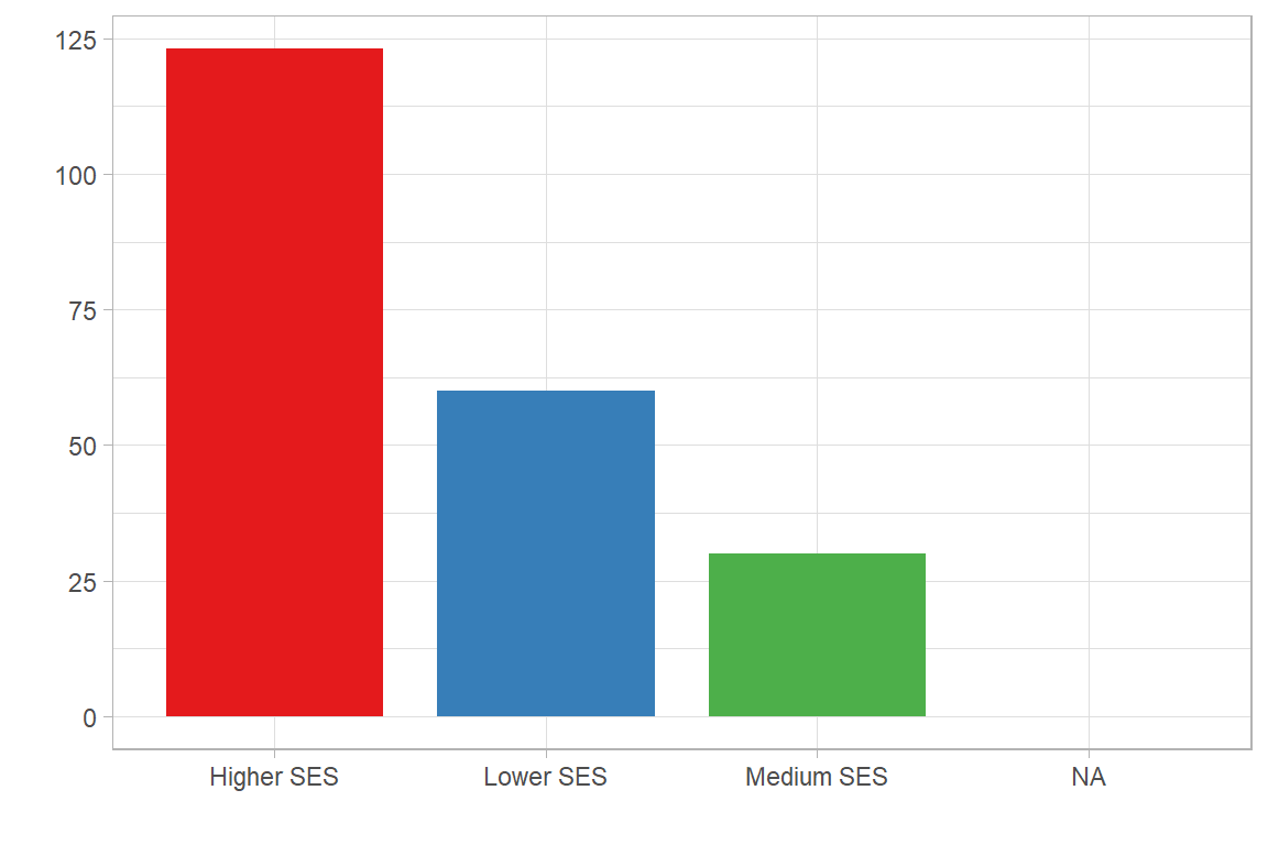

Figure 2.7: Bar chart of ses_3g - Socioeconomic (parents) status

2.2 Working conditions

Respondents can also be characterised by their working conditions, including job position (WCJC001), teaching duties (WCJC023), leadership responsibilities (WCJC027), type of contracts (WCJC010 and WCJC011), salary (WCJC005) and complementary bonus bonus (WCJC005a). Combined with the main socio-demographic variables described in the previous section, the crossing of working condition variables with the main dimensions of social discrimination such as gender, age, socioeconomic status, sexual orientation, health, and ethnic minority status provides the basic groupings to be exploreding in an initial equality audit.

2.2.1 Job position

Code	Question	Responses
WCJC001	What is your current position in the organization you work for?	[1] Academic / researcher [2] Technician [3] Administrative staff

The categorization of staff categories follows Frascati Manual classification of R&D personnel (OECD 2015, 161ff).

df.geam01 |>
  table_frq(WCJC001) 

WCJC001	N	Raw%	Valid%	Cum%
Academic / researcher	143	0.61	0.66	0.66
Technician	31	0.13	0.14	0.81
Administrative	39	0.17	0.18	0.99
Other	3	0.01	0.01	1.00
NA	17	0.07	0.00	1.00

Table 2.15: Frequency table of WCJC001 - Job position

GEAM version 3 has follow-up questions inquiring about more fine-grade categories within each of these job positions (WCJC024 - for Academics/researchers, WCJC025 - for Technicians, and WCJC0026 - for Administrative staff).

One would expect that women are overrepresented among administrative personnel while the gender represenattion should be more equal at the academic level (depending on age) and for technicians. In the following code, we also remove all NAs from both the gender as well as job position variable:

cpal <- RColorBrewer::brewer.pal(3, "Set1")

df.geam01 |>
    filter(!is.na(WCJC001) & !is.na(SDEM004.bin)) |>
    ggplot(aes(x=WCJC001, fill=SDEM004.bin)) + 
    geom_bar(width=.8, 
             position=position_dodge()) +
    geom_text(stat='count', 
              aes(label=after_stat(count)), 
              position=position_dodge(width=.8), 
              vjust=-.6) +
    scale_fill_manual(values=cpal) +
    ylim(0,100) +
    labs(x="Job position", y="", fill="Gender") +
    theme_light()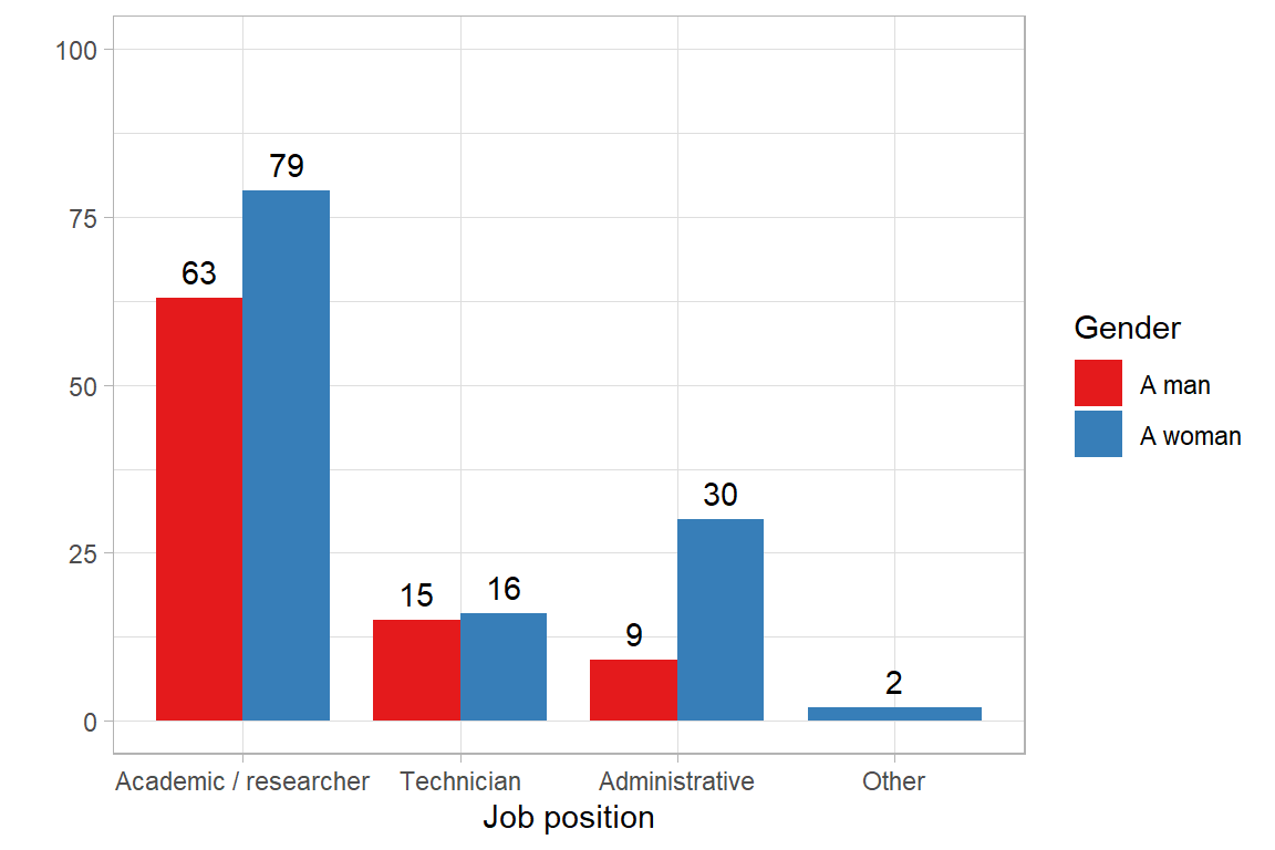

Figure 2.8: Gender by job position bar chart

Women are over-represented among administrative staff, as can be expected. Vertical segregation should be visible when examining academic positions more closely.

2.2.2 Teaching duties

A simple question asks about teaching duties of resondents (variable WCJC023).

Warning

Available datasets do not contain this variable!

2.2.3 Leadership position

Question WCJC027 asks about the number of people that report to the respondent. This indicates leadership responsibilities.

Code	Question	Response
WCJC027	How many people do directly and indirectly report to you?	[1] 0 [2] 1 - 5 [3] 6 - 10 [4] 11 - 20 [5] 21 - 50 [6] More than 50

Warning

Available datasets do not contain this variable!

2.2.4 Type of contract

The type of contract of respondents is covered by two separate questions. Whereas WCJC010 inquires about full-/or part-time contract, WCJC011 inquires about permanent vs. temporary contracts.

Code	Question	Responses
WCJC010	Are you on a full- or part-time contract?	[1] Part-time [2] Full-time [3] Other:

df.geam01 |>
  table_frq(WCJC010) 

WCJC010	N	Raw%	Valid%	Cum%
Part-time	8	0.03	0.04	0.04
Full-time	203	0.87	0.94	0.98
Other	4	0.02	0.02	1.00
NA	18	0.08	0.00	1.00

Table 2.16: Frequency table of WCJC010 part-time/full-time contract

And fixed-term/temporary contract?

Code	Question	Responses
WCJC011	Are you on a permanent/open-ended or fixed-term/temporary contract?	[1] Fixed-term / temporary [2] Permanent / open-ended [3] Other:

df.geam02 |>
  table_frq(WCJC011)

WCJC011	N	Raw%	Valid%	Cum%
Fixed-term/temporary	31	0.28	0.36	0.36
Permanent/open-ended	56	0.51	0.64	1.00
NA	22	0.20	0.00	1.00

Table 2.17: Frequency table of WCJC011 open-ended or temporay contract

Type of contract, especially in terms of permanent versus fixed-term should be explored in relation to different socio-demographic variables, as it is an important indicator of precarious working conditions (European Commission 2021). Section 3.1.2 introduces the statistical techniques to detect if gender differences by type of contract are significant.

2.2.5 Salary

WCJC005	N	Raw%	Valid%	Cum%
Less than €1,000	6	0.03	0.03	0.03
€1,000 - €1,999	111	0.48	0.53	0.55
€2,000 - €2,999	68	0.29	0.32	0.88
€3,000 - €3,999	10	0.04	0.05	0.92
€4,000 - €4,999	9	0.04	0.04	0.97
€5,000 - €5,999	6	0.03	0.03	1.00
€7,000 - €7,999	1	0.00	0.00	1.00
NA	22	0.09	0.00	1.00

Table 2.18: Frequency table of WCJC005 - Salary

References

APA. 2007. “Report of the APA Task Force on Socioeconomic Status.” American Psychological Association.

European Commission. 2021. “MORE4: Support Data Collection and Analysis Concerning Mobility Patterns and Career Paths of Researchers : Survey on Researchers in European Higher Education Institutions.” LU: Publications Office.

Guyan, Kevin, Amanda Aldercotte, Jörg Müller, Maria Caprile, and Sergi Yanes Torrado. 2022. “The Development of the Gender Equality Audit and Monitoring Survey.” In A Community of Practice Approach to Improving Gender Equality in Research, edited by Rachel Palmen and Jörg Müller, 44–63. London ; New York: Routledge. https://doi.org/10.4324/9781003225546-3.

OECD, ed. 2015. Frascati Manual 2015: Guidelines for Collecting and Reporting Data on Research and Experimental Development. The Measurement of Scientific, Technological and Innovation Activities. Paris: OECD.

Stadler, Gertraud, Marie Chesaniuk, Stephanie Haering, Julia Roseman, Vera Maren Straßburger, Schraudner Martina, Ahmad Aisha-Nusrat, et al. 2023. “Diversified Innovations in the Health Sciences: Proposal for a Diversity Minimal Item Set (DiMIS).” Sustainable Chemistry and Pharmacy 33 (June): 101072. https://doi.org/10.1016/j.scp.2023.101072.

UNESCO Institute for Statistics. 2012. International Standard Classification of Education (ISCED) 2011. Montreal QC, Canada: UNESCO Institute for Statistics. https://doi.org/10.15220/978-92-9189-123-8-en.