5 Compare organisations

Author

Affiliation

Dalia Argudo

Abstract

This chapter presents a methodological framework for conducting comparative analyses of gender gaps using data from the GEAM survey. Its objective is to guide practitioners in identifying and examining gender disparities in working conditions, work–life balance, organisational perceptions, and experiences of discrimination across faculties, departments, or organisations. The examples are drawn from three research organisations based in different countries; however, detailed contextual information about each national setting is not used for the analytical approach presented here.

Keywords

Compare organisations, Gender gaps

Comparing gender gaps across organisations is a key tool for understanding how different workplace environments can influence gender inequalities. Beyond identifying internal disparities, this type of analysis enables the observation of structural patterns, the recognition of institutional good practices, and the design of more targeted and evidence-based interventions. In the context of the GEAM survey, such comparisons are particularly useful for highlighting differences in working conditions, work–life balance, organisational perceptions, and experiences of discrimination, among other relevant dimensions.

This chapter presents a practical methodological framework for conducting comparative analyses using GEAM survey data. It can be applied in diverse institutional contexts—such as faculties, departments, or research centres—and even across organisations based in different countries. Although the analysis is illustrated using data from three international organisations, detailed knowledge of the national context of each is not required in order to effectively carry out the comparison. The proposed approach is structured around a series of stages that guide the user from descriptive profiling to adjusted statistical modelling, providing a deeper understanding of potential inequalities.

The following chapter will outline each step of the analytical process, from the preparation and cleaning of the data to the visualisation of results and reporting of findings. Throughout, guidance will be offered on how to tailor the approach to different organisational levels, which techniques to use at each stage, and how to interpret findings with a critical and action-oriented lens.

This comparative framework is intended as a practical tool for those involved in designing and implementing gender equality plans. It enables practitioners to identify which organisations present more equitable conditions, where the most significant inequalities are found, and which individual or structural factors are associated with these outcomes. Furthermore, it supports the identification of good practices—such as effective work–life balance measures, inclusive policies, or positive organisational climates—that can serve as models for other institutions. Systematic comparison of results not only helps to expose gaps but also to recognise and disseminate successful approaches that contribute to more inclusive and equitable work environments.

5.1 Stage 1. Preparation and cleaning of multiple bases

This initial stage lays the foundation for any robust and meaningful comparative analysis. Before conducting any descriptive or inferential statistics, it is essential to ensure that the data from different organisations (or departments, faculties, etc.) are compatible, and harmonised.

5.1.1 Why this stage matters

Comparing gender equality data across multiple organisational contexts requires particular attention to data integrity and consistency. Differences in variable formats, coding schemes, or missing values can compromise the comparability of results. Therefore, harmonisation and cleaning must be undertaken before analysis begins.

This step is especially crucial when:

You are working with data from different countries, institutional structures, or administrative systems.
You want to compare data across levels (e.g., organisation-wide vs. by faculty or department).
You are using GEAM datasets collected independently by each organisation or unit.

5.1.2 Merge data sources

If each organization or unit has its own data set, it will be necessary to combine them into a single database.

The first step will be to create a new categorical variable (e.g., organisation_id or unit_id) that identifies the origin of each case.

For this case, we have three datasets from different organisations and we will create the variable org with a label that identifies each dataset.

# Step 1.1 — Create a column (variable) that identifies the organisation
df.geam01$org <- "org_01"
df.geam02$org <- "org_02"
df.geam03$org <- "org_03"

Listing 5.1: Organisation identifier variable

Note

If the comparison is within a single organisation, such as between departments or faculties, the categorical variable should identify those internal units.

To make meaningful comparisons, we need to ensure that the variables across datasets share the same names, formats, and measurement scales. Therefore, the following next step is to review and harmonise variables.

The GEAM core questionnaire ensures that the variables have the same names, formats, and measurement scales. However, it is a customizable survey, and some organisations may have added variables or modified core variables to suit their specific contexts.

Note

Some organisations may have conducted multiple GEAM surveys over time, potentially using different versions of the questionnaire. In such cases, harmonising variables becomes necessary to facilitate comparisons across time (see Chapter 4).

In our case, the variables SDEM001andSDEM012 in one of the datasets were modified and collect different information than the other datasets. Therefore, we will rename these variables to distinguish them from the originals.

Click to see the code to check levels and rename variables

# Step 1.2 - Check levels of variables
unique(df.geam01$SDEM001)
#> [1] 35-44       25-34       45-54       55-64       18-24       <NA>       
#> [7] 65 or older
#> Levels: 18-24 25-34 35-44 45-54 55-64 65 or older
unique(df.geam01$SDEM012)
#>  [1] South America   Western Europe  Eastern Europe  Southern Europe
#>  [5] Middle East     <NA>            Southeast Asia  South Asia     
#>  [9] Other           North America   East Asia       Central America
#> [13] Northern Europe Caribbean      
#> 17 Levels: Eastern Europe Western Europe Central Asia ... Other

# Rename variables SDEM001 and SDEM012 
df.geam01 <- df.geam01 %>% rename(SDEM001_cat = SDEM001)
df.geam01 <- df.geam01 %>% rename(SDEM012_region = SDEM012)

In addition, we will create an approximation of the variable age for the databased (org_01) which do not have the question about the respondent’s year of birth (SDEM001).

Show the code to create continuous variable

# Create a continuous variable age (midpoint imputation)
df.geam01 <- df.geam01 %>%
  mutate(
    age = case_when(
      SDEM001_cat == "18-24" ~ 21,
      SDEM001_cat == "25-34" ~ 29.5,
      SDEM001_cat == "35-44" ~ 39.5,
      SDEM001_cat == "45-54" ~ 49.5,
      SDEM001_cat == "55-64" ~ 59.5,
      SDEM001_cat == "65 or older" ~ 67,   
      TRUE ~ NA_real_
    )
  )

For the purposes of comparison, only common variables can be used. Therefore, we begin by identifying the variables shared across the organisations and retain only those. These will then be merged into a single, unified dataset.

# Step 1.3 - Unify common columns (variables) between databases
# Finding common variables
common_vars <- Reduce(intersect, list(names(df.geam01), names(df.geam02), names(df.geam03)))

# Keeping only common variables for comparative analysis
df.geam01_common <- df.geam01[, common_vars]
df.geam02_common <- df.geam02[, common_vars]
df.geam03_common <- df.geam03[, common_vars]

# Step 1.4 — Unify the databases into a single data frame
df.combined <- bind_rows(df.geam01_common, df.geam02_common, df.geam03_common)

Listing 5.2: Merge databases

5.1.3 Missing data

Another important step is identifying missing data. This can help detect nonresponse patterns across questions or organisations. For example, if many people fail to respond to questions about salary or harassment, this may reflect not only missing data but also a cultural or institutional issue.

Evaluating missing data also help avoid bias in the results if the missing values are not random. For example, if there are more missing data for women or within a given organisation, the analyses may overestimate or underestimate averages or generate erroneous inferences.

First, we will obtain a general pattern of missing values through graphs.

Show code for producing the following figure

library(naniar)
vis_miss(df.combined, cluster = TRUE)

Figure 5.1: Binary heat map of NA values

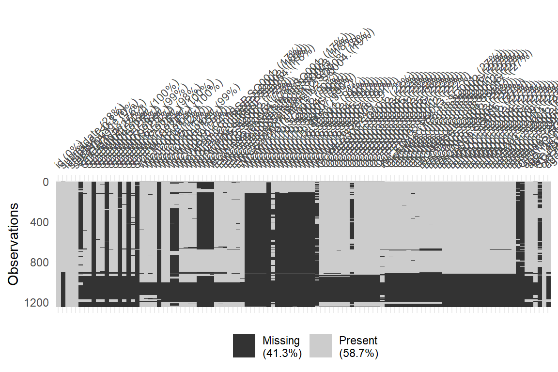
The Figure 5.1 shows a binary heat map where each row represents an observation (respondent) and each column represents a variable (question). Gray cells indicate present values (not NA) and dark cells indicate missing values (NA).

Show code for producing the following figure

gg_miss_upset(df.combined)

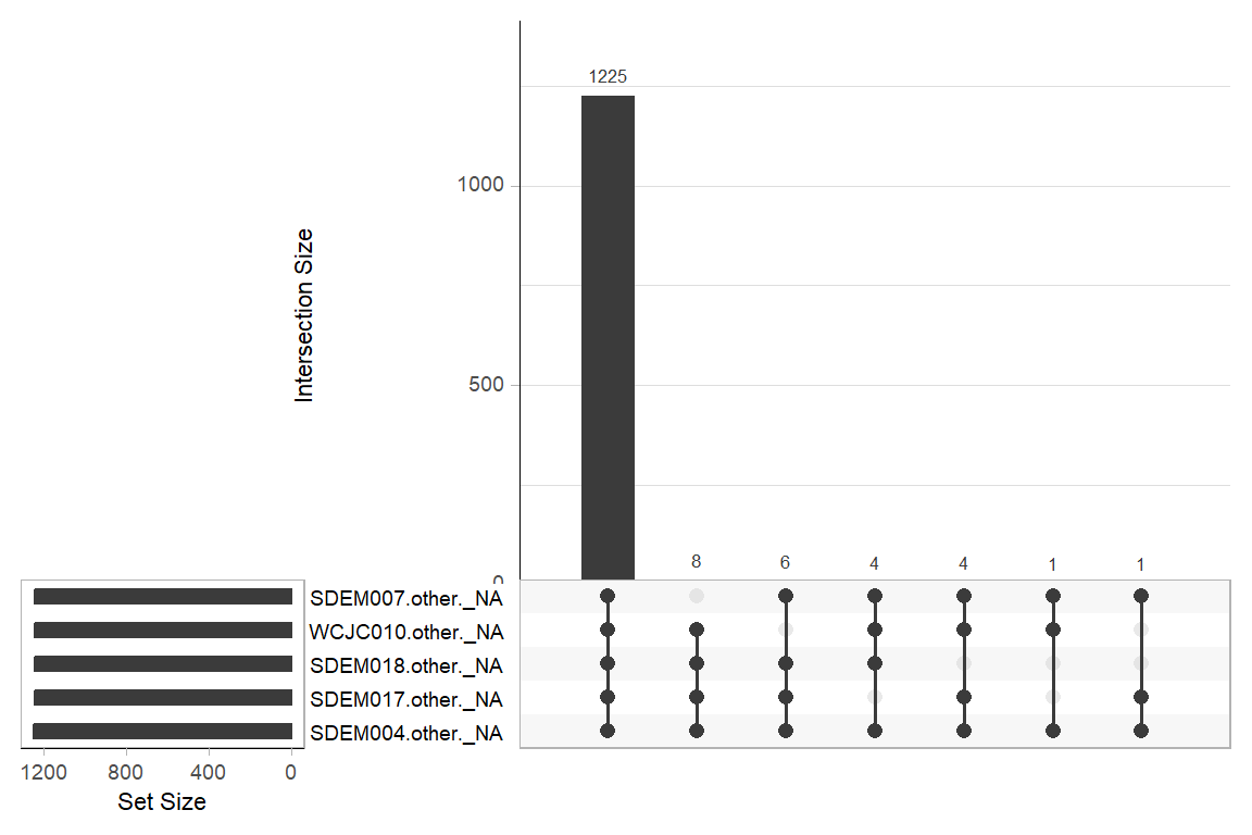
Figure 5.2: Overall pattern of NA values

The Figure 5.2 shows which variables tend to have missing values at the same time, and how many cases follow each missing data pattern. In this dataset, the most common pattern involves questions labeled as ‘Other’ these are follow-up questions that only appear when a respondent selects Other as a response to a previous question (e.g., level of education). Since most respondents choose predefined options, it is expected that the majority of these Other (specify) questions are missing (NA) by design.

Next, we will break down the missing data by organisation. To do this, we will generate a table that displays the percentage of missing values for each variable across different organisations.

Show code for producing the following table

library(dplyr)
library(tidyr)
library(naniar)

# Step 1.4 — Identify missing data
# Creating a  table that shows missing by variable and organisation
df.combined |>
  group_by(org) |>
  miss_var_summary() |>
  head(10) |>
  kable()

org	variable	n_miss	pct_miss
org_01	SDEM004.other.	233	100
org_01	WCWI011b.other.	233	100
org_01	SDEM017.other.	232	99.6
org_01	SDEM018.other.	232	99.6
org_01	SDEM007.other.	231	99.1
org_01	SDEM016.other.	229	98.3
org_01	WCJC010.other.	229	98.3
org_01	GEAMCOM	218	93.6
org_01	BISB005	217	93.1
org_01	WCWI023	214	91.8

Table 5.1: Percentage of NA by variable and organisation

Note

Note that table only displays the first 10 results after using head(10). Alternatively, you can filter by a given percentage of missing values and set a minimum coverage for the analysis. For example, less than 35% of missing values filter(pct_miss < 35)

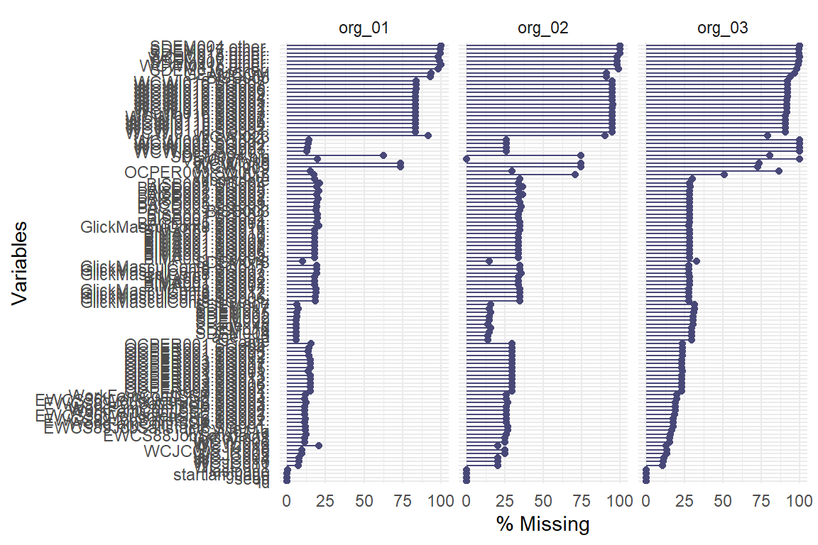
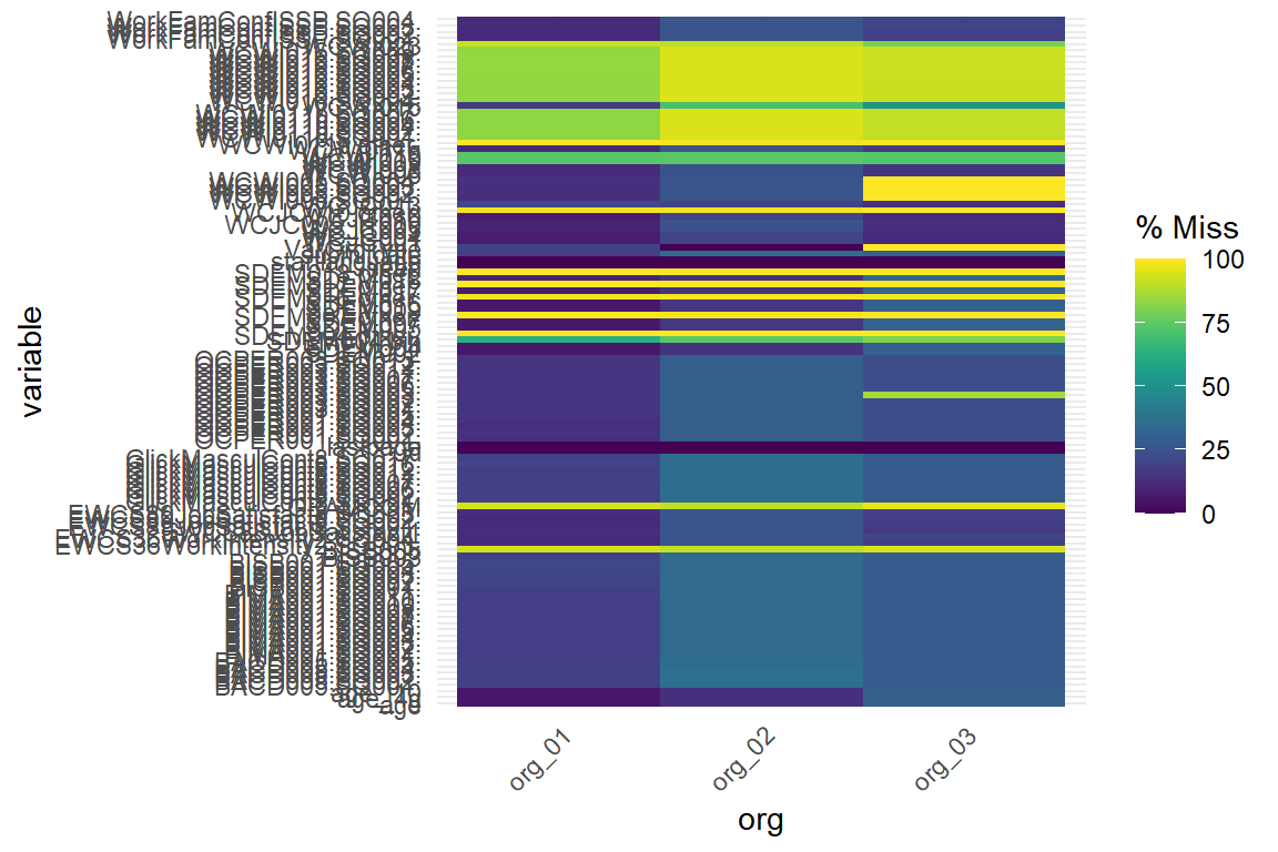
It is also possible to explore the percentage of missing values by variable and organisation (or any other classification variable) through graphs.

Show code for producing the following figure

#Visualise missing data
gg_miss_var(df.combined, facet = org, show_pct=TRUE)

Figure 5.3: Percentage of NAs by organisation

Show code for producing the following figure

#Visualise missing data
gg_miss_fct(x = df.combined, fct = org)

Figure 5.4: Heat map of NA values by organisation

From the Table 5.1 or Figure 5.3 or Figure 5.4, we can distinguish whether a variable has more NAs in one organisation compared to the others. This indicates that the quality or availability of data for that variable depends on the organisation.

For example, in our database, we can see that org_3 has a higher percentage of missing data for some variables compared to the other two organisations. This could be due to reasons such as data collection issues or the variable not being applicable to the context.

Note

This section covers only part of the missing data analysis. For a more detailed overview of handling missing data in R, please see this link.

5.1.4 Derived variables and indices

The next step, of this stage will be to create derived variables and indices. The Chapter 8 and Chapter 9 provide a guide to create outcome varibles of interest (e.g., index of work-life balance).

This is also the stage to transform continuous variables into categories (e.g., age groups Listing 2.5) or create dichotomous variables (e.g., binary gender variable Listing 2.3).

We are going to calculate the following variables and indices:

Binary gender (Listing 2.3)

Show code to create the variable

# Create binary gender variable
df.combined <- df.combined |>
  mutate(SDEM004.bin = case_when(
    SDEM004 == "Prefer not to say" ~ NA,
    SDEM004 == "Non-binary" ~ NA, 
    SDEM004 == "Other" ~ NA,
    .default = SDEM004
  ))

Socioeconomic status (Listing 2.6 and Listing 2.7)

Show code to create the variable

# create new SES variable based upon the higher value of SDEM017 vs. SDEM018
df.combined <- df.combined |>
  mutate(SDEM017.comp = if_else(SDEM017 == "Prefer not to say" | 
                                SDEM017 == "Other" | 
                                is.na(SDEM017), -99, as.numeric(SDEM017)), 
         SDEM018.comp = if_else(SDEM018 == "Prefer not to say" |
                                SDEM018 == "Other" | 
                                is.na(SDEM018), -99, as.numeric(SDEM018)), 
         higher_ses = if_else(SDEM017.comp >= SDEM018.comp, SDEM017.comp, SDEM018.comp))

# create three SES groups
df.combined <- df.combined |>
  mutate(ses_3g = case_when(
    higher_ses >0 & higher_ses <=3 ~ "Lower SES", 
    higher_ses >3 & higher_ses <=5 ~ "Medium SES",
    higher_ses >5 & higher_ses <=9 ~ "Higher SES",
    .default = NA
  ))

# reconvert to factor
df.combined$ses <- factor(df.combined$ses_3g)

Care responsibilities (Listing 8.1)

Show code to create the variable

# Create binary care responsibilities
df.combined<-df.combined |> 
        mutate(CareResp = if_else((WCWI006 == "Yes" | 
                                   WCWI008 == "Yes"), TRUE,FALSE))

Level of education three groups (Listing 3.4)