4 A comparative analysis over time

This chapter analyses changes in the perception of gender equality at the National Information Processing Institute in Poland between 2020 and 2024. The study is based on two rounds of monitoring conducted using the GEAM tool. Scales that measure work culture, masculinity contest culture, microaggressions, equality practices, and the redistribution of resources and responsibilities were considered. The findings indicate an overall improvement in workplace culture and perceptions of gender equality—although women remain less likely to view the institute as one that ensures equal treatment. Despite the implementation of equality-promoting policies, gender disparities in perceived access to resources and responsibilities persist. No significant changes were observed in the perception of masculinity contest culture and the frequency of microaggressions; however, the data reveals that microaggressive behaviour was less frequent in 2024. These results indicate the potential positive impact of institutional policies and changes in work organisation after the COVID-19 pandemic on perceived equality, which underscores the need for continued monitoring and long-term evaluation.
gender equality plan, gender equality audit, equality data monitoring, GEAM tool, statistical analysis
4.1 Introduction - Gender equality at a research institute, a comparative analysis over time
The National Information Processing Institute (OPI PIB) is a Polish research centre dedicated to supporting science and higher education policy. What sets OPI PIB apart as a scientific institution is its dual role: in addition to conducting research, it also operates as a software house, developing IT systems that are tailored to the needs of the Polish science and higher education sectors. As a result, the largest group of employees consists of engineering and technical staff, with men comprising nearly 60% of that group.
In 2020, OPI PIB implemented a survey-based gender equality audit using the GEAM tool. The study, titled Monitoring of Working Conditions, Safety, and Equal Treatment, had three main objectives. First, it aimed to assess OPI PIB employees’ perceptions of their workplace. This included understanding how the institute’s workforce viewed their employer and career prospects, as well as whether they had experienced harassment or unequal treatment. It also involved gathering insights into their opinions on gender equality at the institute. Second, the study sought to analyse employees’ experiences during the COVID-19 pandemic. Conducted in October 2020, at the height of the pandemic, the study explored employees’ experiences with remote work, changes in their wellbeing (both improvements and declines), and evaluation of the support provided by the employer during that period. The study’s third objective was to support initiatives that aim to advance gender equality in Central and Eastern Europe (CEE). OPI PIB contributed actively to the Community of Practice for Gender Equality in CEE under the ACTonGender project. That study aimed to provide insights that could drive broader changes in gender equality across the region.
The COVID-19 pandemic brought changes in the work environment and has had a lasting impact on many institutions, including those in the science and higher education sectors. Many aspects of professional life moved online; communication both within and between teams shifted predominantly to online meeting platforms (Pabilonia and Redmond 2024). Remote work, initially introduced as a reaction to the pandemic, has become a permanent feature. In April 2023, new regulations that govern the practice were implemented in Poland. Poland’s Labour Code defined remote work and outlined its principles, which led to the introduction of new organisational work policies at many institutions, including OPI PIB. The policy at OPI PIB established remote work limits for individual departments and teams: up to 90% remote work for employees primarily engaged in software development and research; and up to 70% remote work for employees primarily involved in user support, administration, or finance. Currently, all of OPI PIB’s employees work remotely to some extent, with over 70% of the workforce working 90% of their time in that mode. On one hand, remote work has made it easier for employees who are based in locations other than Warsaw to join OPI PIB, thus expanding the institute’s talent pool. On the other, it has introduced challenges, such as work intensification, poor adaptation to new ways of working from home, staff interactions, and the need for employees to create home workspaces and to balance work with family responsibilities (Adisa, Ogbonnaya, and Adekoya (2021), Alfano et al. (2024)).
In the autumn of 2024, the GEAM survey was repeated, with the primary goal of assessing the changes that had occurred during the previous four years. This evaluation considered significant transformations at the institute, including a notable increase in employment (from just under 400 in 2020 to over 500 staff in 2024), the introduction of a gender equality plan (2022), and the appointment of an equality officer who is tasked with coordinating measures for equal treatment (2023).
4.2 Methods
4.2.1 Data collection and sample structure
Both waves of the study were conducted using online questionnaires. Invitations to participate were sent by email to all OPI PIB employees, alongside a link to the questionnaires on LimeSurvey.
The two editions differed in terms of their numbers of respondents. In 2020, a total of 152 employees participated in the study, of which sixty-three completed the entire questionnaire. In 2024, 308 respondents participated, with 180 completing the entire questionnaire. This chapter analyses all responses, not only the completed questionnaires.
In a first pre-processing step, the two datasets for 2020 and 2024 need to be merged, unifying variable names in the process. We basically add the rows from 2020 and 2024 into a single dataset, selecting only those predictor variables we are interested in, namely gender, managerial position, parent status, and job position. An additional column year is added, to indicate the respective year of a response.
# remove variable names
attr(df.geam20, "variable.labels") <- NULL

# define color palette
cpal <- RColorBrewer::brewer.pal(6, "Set1")

# rename variables of 2020 dataset and add 'year' column 2020
df20 <- df.geam20 |>
  select(gender = SDEM004,      # gender
         manager = G01Q65,      # managerial position
         parent = WCWI008,      # parent / legal guardian of a child / children
         position = WCJC001) |> # Job position
  mutate(year = 2020)

# rename multi-item questions, removing '.' at the end
# for easier selection later on
df.geam24 <- df.geam24 |>
  rename_with(~ str_sub(.x, end=-2), contains(".SQ"))


# rename variables of 2024 dataset and add 'year' column 2024
df24 <- df.geam24 |>
  select(gender = SDEM004,      # gender
         manager = WCJC026,     # level of position
         parent = WCWI008,      # parent or legal guardian of a child / children
         position = WCJC001) |> # Job position
  mutate(year = 2024)

# combine 2020 and 2024 datasets into a new one
df.geam20.24 <- bind_rows(df20, df24) |>
mutate(year = as.factor(year))After merging, Table 4.1 provides a quick overview of the summary statistics of our main variables grouped by the year.
df.geam20.24 |>
  tbl_summary(include = c(gender, manager, parent),
              by=year,
missing_text = "(Missing)")| Characteristic | 2020 N = 1521 |
2024 N = 3081 |
|---|---|---|
| gender | ||
| A man | 56 (48%) | 103 (39%) |
| A woman | 53 (45%) | 139 (52%) |
| I do not want do answer | 8 (6.8%) | 0 (0%) |
| Non-binary | 0 (0%) | 3 (1.1%) |
| Prefer not to say | 0 (0%) | 17 (6.4%) |
| Other | 0 (0%) | 4 (1.5%) |
| (Missing) | 35 | 42 |
| manager | ||
| Yes | 15 (15%) | 0 (0%) |
| No | 85 (83%) | 0 (0%) |
| Prefer not to say | 3 (2.9%) | 0 (0%) |
| Director, deputy director, manager, leader | 0 (0%) | 30 (13%) |
| Independent specialist, chief specialist | 0 (0%) | 57 (24%) |
| Senior specialist, experienced specialist | 0 (0%) | 124 (53%) |
| Junior specialist | 0 (0%) | 23 (9.8%) |
| (Missing) | 49 | 74 |
| parent | ||
| Yes | 36 (42%) | 99 (45%) |
| No | 44 (52%) | 109 (50%) |
| Prefer not to say | 5 (5.9%) | 11 (5.0%) |
| (Missing) | 67 | 89 |
| 1 n (%) | ||
However, as we can see in the above table, response options also differ between the 2020 and 2024 datasets (note how some items have uniformly zero responses on the left vs. right column) and need to be matched.
df.geam20.24 <- df.geam20.24 |>
  mutate(
      gender = case_when(
      gender == "I do not want do answer" ~ NA,
      gender == "Non-binary" ~ NA,
      gender == "Prefer not to say" ~ NA,
      gender == "Other" ~ NA,
      .default = gender
    ),
      manager = case_when(
      manager == "Prefer not to say" ~ NA,
      manager == "Director, deputy director, manager, leader" ~ "Yes",
      manager == "Independent specialist, chief specialist" ~ "No",
      manager == "Senior specialist, experienced specialist" ~ "No",
      manager == "Junior specialist" ~ "No",
      .default = manager),
      parent = case_when(
      parent == "Prefer not to say" ~ NA,
      .default = parent)
    )|>
  mutate(
    gender = fct_drop(gender),
    manager = fct_drop(manager),
    parent = fct_drop(parent)
)After matching and thus unifying the response options across both years, Table 4.2 now provides summary statistics of our main predictor variables by years.
df.geam20.24 |>
  tbl_summary(include = c(gender, manager, parent),
              by=year,
              type = all_dichotomous() ~ "categorical",
              digits = everything() ~ c(0,1),
missing_text = "(Missing)")| Characteristic | 2020 N = 1521 |
2024 N = 3081 |
|---|---|---|
| gender | ||
| A man | 56 (51.4%) | 103 (42.6%) |
| A woman | 53 (48.6%) | 139 (57.4%) |
| (Missing) | 43 | 66 |
| manager | ||
| No | 85 (85.0%) | 204 (87.2%) |
| Yes | 15 (15.0%) | 30 (12.8%) |
| (Missing) | 52 | 74 |
| parent | ||
| Yes | 36 (45.0%) | 99 (47.6%) |
| No | 44 (55.0%) | 109 (52.4%) |
| (Missing) | 72 | 100 |
| 1 n (%) | ||
In terms of gender, the 2020 sample was quite evenly split between men and women, with a slight male majority; in 2024, however, female respondents were more numerous than male ones (see Table 4.2). The samples were similar regarding the respondents’ current positions at OPI PIB. At both time points, the majority (approximately 60%) worked in technical roles, with approximately one in four in administrative positions (27.2% in 2020 and 25.2% in 2024). Researchers comprised approximately 14% of both samples. The proportion of respondents who held managerial positions differed only slightly between the two years, with a higher share in 2020 (15.0% vs. 12.8% in 2024). The samples were also similar in terms of the proportion of parents or legal guardians of children under eighteen years, with slightly higher shares of individuals without children (51.8% in 2020 and 49.8% in 2024).
4.2.2 Dependent Variables
For the purposes of the analysis, we constructed scales that measure: work culture OCWC002, masculinity contest culture MCC (Glick, Berdahl, and Alonso 2018), respondents’ experiences of microaggressions at work BIMA001, overall perceptions of equality practices at the institute OCPER001, and the redistribution of resources and responsibilities OCPER003. For each scale, we selected items from a relevant group of questions that were adequate and comparable between the two surveys. For comparable items worded in the opposite way, reverse coding was applied.
See Section 4.6 for details for wording of sub-question items in both surveys, the coding applied, and the Cronbach’s alpha values for each case.
There was also a difference in the wording between the two surveys of the questions on respondent’s experiences of microaggressions at work BIMA: in 2020, we asked about experiences ‘at the workplace’; in 2024, we asked specifically about employees’ experiences at OPI PIB. This nuance must be considered when interpreting the results. The broader scope of the 2020 question might have led to inconsistencies due to possible multiple-employer situations or references to previous jobs.
The internal consistency of each scale was tested using the Cronbach’s Alpha coefficient. The results of the reliability assessment were satisfactory, with the lowest alpha values observed in the OCPER001 group: 0.70 in 2020 and 0.76 in 2024.
4.2.3 Data analysis
This analysis examines the MCC, OCWC002, BIMA001, OCPER001, and OCPER003 scales using data from GEAM 2020 and GEAM 2024. To harmonise the responses in both years, numerical coding was applied as follows:
- OCWC002, MCC, OCPER001, and OCPER003: scale from −2 to 2
- BIMA: scale from 0 to 3.
The key demographic variables included are:
- Gender
- Managerial status
- Parental status
For each scale, a composite index was calculated by averaging the responses to all relevant survey items for each respondent. This approach created a single numerical measure that represents the overall score for the scale.
Mean analysis
To assess trends over time, mean scores were calculated for each group: 1) men (2020), 2) women (2020), 3) men (2024), and 4) women (2024). A bar plot was generated for each scale, which illustrates the mean scores across gender and survey year.
Regression analysis
Model Specification
A progressive modeling approach was adopted to examine how the Index (the dependent variable) was influenced by time and key categorical factors, and whether these relationships changed between 2020 and 2024. The model was constructed in stages with groups of predictors added sequentially. A simple model containing only a time indicator was estimated first, followed by the inclusion of main effects of categorical variables, and finally, interaction terms were incorporated.
Because the data consist of two independent cross-sectional samples, a binary indicator variable, year2024, was included to distinguish observations from 2024 (coded 1) versus the 2020 baseline (coded 0). The three models described below were specified to reflect this progression, with the interpretation of model terms outlined accordingly.
Model 1: Base Model (Year Effect Only)
The first model was specified with year2024 as the only explanatory variable. This model was used to test whether a difference in Index scores existed between the two survey years, without accounting for any other variables. It was formally expressed as: \[ \text{Index}_i = \beta_0 + \beta_1 \, \text{year2024}_i + \varepsilon_i \]
In this specification:
\(\beta_0\) represents the mean Index score in 2020 (the reference year),
\(\beta_1\) captures the average difference in the Index in 2024 relative to 2020,
\(\varepsilon_i\) denotes the residual error for observation \(i\).
Model 2: Main Effects Model
In the second model, the main effects of gender, managerial role, and parent status were added. This allowed for the assessment of their independent associations with the Index, while also accounting for year. The model was specified as follows: \[ \text{Index}_i = \beta_0 + \beta_1 \, \text{year2024}_i + \beta_2 \, \text{gender}_i + \beta_3 \, \text{manager}_i + \beta_4 \, \text{parent}_i + \varepsilon_i \] In this model:
\(\beta_0\) corresponds to the mean Index score for the reference group (male, non-manager, non-parent) in 2020,
\(\beta_2\), \(\beta_3\), and \(\beta_4\) represent the differences in Index associated with being female, a manager, and a parent, respectively, in 2020,
\(\beta_1\) reflects the effect of year (2024 vs 2020), representing the overall change in Index between 2020 and 2024, regardless of demographic characteristics,,
\(\varepsilon_i\) is the error term, is the error term, accounting for unobserved individual-level variability in Index.
Model 3: Final Model with Interaction Terms (Year × Category Effects)
The final model expanded on Model 2 by incorporating interaction terms between ‘year2024’ and each of the categorical variables. This allowed the effects of gender, managerial role, and parent status on the Index to vary between 2020 and 2024. The full model is expressed as: \[ \text{Index}_i = \beta_0 + \beta_1 \text{gender}_i + \beta_2 \text{year2024}_i + \beta_3 (\text{gender}_i \times \text{year2024}_i) + \beta_4 \text{manager}_i + \\ \beta_5 (\text{manager}_i \times \text{year2024}_i) + \beta_6 \text{parent}_i + \beta_7 (\text{parent}_i \times \text{year2024}_i) + \varepsilon_i \] where:
\(\beta_0\) represents the baseline level of Index for the reference category of each predictor in 2020.
\(\beta_1\), \(\beta_4\), and \(\beta_6\) capture the main effects of gender, manager, and parent, respectively, in 2020.
\(\beta_2\) indicates the effect of
year2024, reflecting whether there is a systematic difference in Index between 2020 and 2024, independent of other variables.\(\beta_3\), \(\beta_5\), and \(\beta_7\) measure the interaction effects between
year2024and each categorical predictor. A statistically significant coefficient for these terms would indicate that the relationship between Index and the corresponding categorical variable has changed between 2020 and 2024.\(\varepsilon_i\) represents the error term, capturing unobserved factors affecting Index.
Model diagnostics
To evaluate the assumptions of the generalized linear model (GLM), the Breusch–Pagan test was conducted to assess homoscedasticity.
For OCWC002, MCC, BIMA001, OCPER001, and OCPER003, statistically significant deviations from normality were observed.
4.3 Results
4.3.1 Masculinity contest culture (MCC)
4.3.1.1 Preparation and transformation of data
The Masculinity Contest Culture scale contains eight items (see Table 4.29) in both waves. In order to calculate the mean value for each respondent, we convert the ordered answer items into numeric values from -2 to 2. Negative values indicate that a given statement is “not true” while positive statements represent that a given statement is true for the work environment. The scale is centered on 0 (“Neither true nor untrue”). We then add the mean score of the MCC to our main data frame.
# convert mcc answers to numeric, center on 0,
# then calculate mean across all 8 items
df20 <- df.geam20 |>
  select(starts_with("GlickMasculCont8"))|>
  map_df(~ {as.numeric(.x) - 3}) |>
  mutate(mcc_mean = rowMeans(across(everything()), na.rm=T)) |>
  select(mcc_mean)

# do the same for 2024 data
df24 <- df.geam24 |>
  select(starts_with("GlickMasculCont8"))|>
  map_df(~ {as.numeric(.x) - 3}) |>
  mutate(mcc_mean = rowMeans(across(everything()), na.rm=T)) |>
  select(mcc_mean)

# add mean mcc scores to main data frame
df.geam20.24 <- bind_rows(df20, df24)  |>
bind_cols(df.geam20.24) 4.3.1.2 Mean analysis: masculinity contest culture
Click to see code for producing MCC mean scores table
df.geam20.24 |>
  select(year, gender, manager, parent, mcc_mean)|>
  drop_na()|>
  tbl_custom_summary(
    by = year,
    include = c(gender, manager, parent),
    stat_fns = everything() ~ function(data, ...){
       m <- mean(data$mcc_mean, na.rm = TRUE)
       tibble(mean_mcc_score = m)
    },
    statistic = everything() ~ "{mean_mcc_score}",
    digits = everything() ~ c(3),
    type = all_dichotomous() ~ "categorical",
    overall_row = T
) |>
  add_overall(last=T)|>
modify_spanning_header(all_stat_cols() ~ "**Mean MCC scores**")| Characteristic |
Mean MCC scores
|
||
|---|---|---|---|
| 2020 N = 571 |
2024 N = 1661 |
Overall N = 2231 |
|
| Overall | |||
| TRUE | -0.842 | -0.859 | -0.855 |
| FALSE | NA | NA | NA |
| gender | |||
| A man | -1.034 | -1.021 | -1.025 |
| A woman | -0.681 | -0.746 | -0.731 |
| manager | |||
| No | -0.798 | -0.849 | -0.836 |
| Yes | -1.109 | -0.921 | -0.971 |
| parent | |||
| Yes | -0.967 | -0.891 | -0.907 |
| No | -0.764 | -0.827 | -0.809 |
| 1 mean_mcc_score | |||
The mean values of MCC in both 2020 (−0.84) and 2024 (−0.86) indicate that, in general, the work environment at OPI PIB is not perceived as one that supports male norms. When divided by gender, both women and men tend to view the environment as one that does not support male norms; however, the means are lower for men (−1.03 vs. −0.68 in 2020, and −1.02 vs. −0.75 in 2024), which indicates that men agree with this conclusion slightly more than women do. The results for both parents and nonparents, and for managers and nonmanagers also support the conclusion that OPI PIB is not perceived as a workplace that rewards masculinity. This perception is quite stable: only slight differences can be observed in the means between 2020 and 2024 for the groups discussed above.
# create barchart of MCC scores by year and gender
df.geam20.24 |>
  select(year, gender, mcc_mean) |>
  drop_na()|>
  group_by(year, gender) |>
  summarize(mean = mean(mcc_mean, na.rm=T)) |>
  ggplot(aes(x=gender, y=mean, fill=year)) +
    geom_bar(position="dodge", stat="identity", width=.5) +
    geom_hline(yintercept = 0, color = "black", linetype = "dashed") +
    scale_fill_manual(values=cpal) +
    scale_y_continuous(limits = c(-2, 2)) +
    labs(x="", y="Mean MCC scores", fill="Year") +
    theme_light()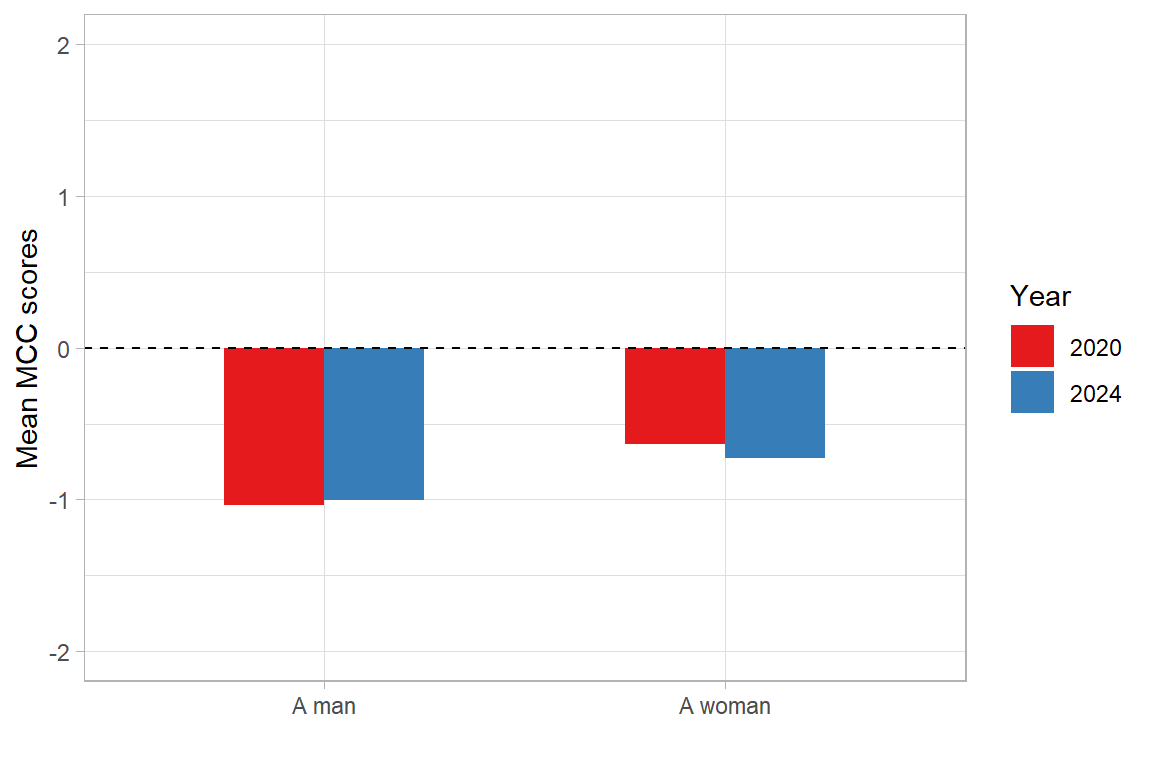
The same information can be presented as a boxplot in Figure 4.2.
# create boxplots for MCC scores by year and gender
df.geam20.24 |>
  select(year, gender, mcc_mean) |>
  drop_na() |>
  ggplot(aes(x=gender, y=mcc_mean, fill=as.factor(year))) +
    geom_boxplot(width=0.5) +
    geom_hline(yintercept = 0, color = "black", linetype = "dashed") +
    scale_fill_manual(values=cpal) +
    scale_y_continuous(limits = c(-2, 2)) +
    labs(x="", y="Mean MCC scores", fill="Year") +
    theme_light()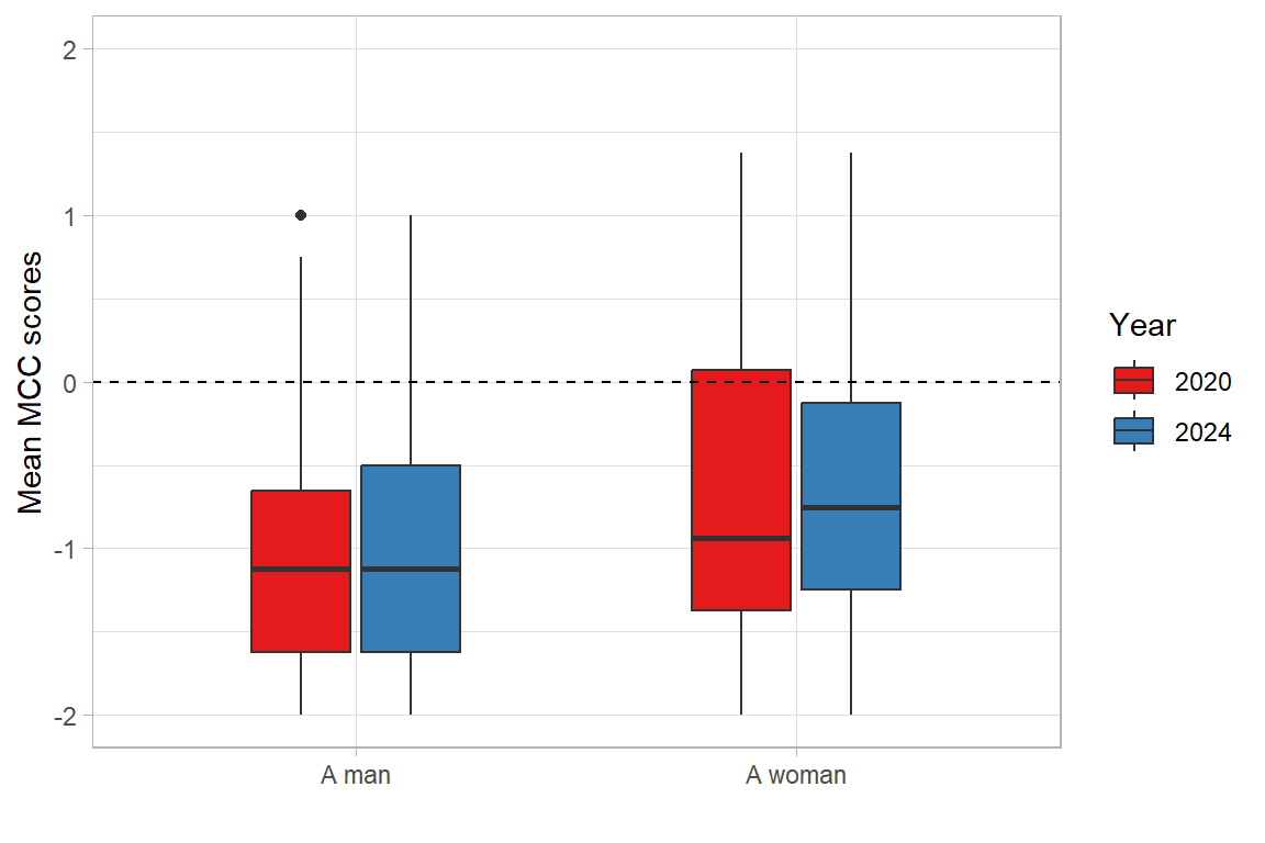
4.3.1.3 Regression analysis: masculinity contest culture
mcc_base <- lm(mcc_mean ~ year, data = df.geam20.24)

mcc_base |>
  tbl_regression(intercept = T,
                 pvalue_fun = label_style_pvalue(digits = 3),) |>
modify_column_unhide(column = c(std.error, statistic)) | Characteristic | Beta | SE | Statistic | 95% CI | p-value |
|---|---|---|---|---|---|
| (Intercept) | -0.84 | 0.102 | -8.30 | -1.0, -0.64 | <0.001 |
| year | |||||
| 2020 | — | — | — | — | |
| 2024 | 0.02 | 0.117 | 0.187 | -0.21, 0.25 | 0.852 |
| Abbreviations: CI = Confidence Interval, SE = Standard Error | |||||
mcc_main <- lm(mcc_mean ~ year + gender + manager + parent, data = df.geam20.24)

mcc_main |>
  tbl_regression(intercept = T,
                 pvalue_fun = label_style_pvalue(digits = 3),) |>
modify_column_unhide(column = c(std.error, statistic)) | Characteristic | Beta | SE | Statistic | 95% CI | p-value |
|---|---|---|---|---|---|
| (Intercept) | -1.0 | 0.132 | -7.72 | -1.3, -0.76 | <0.001 |
| year | |||||
| 2020 | — | — | — | — | |
| 2024 | -0.02 | 0.119 | -0.208 | -0.26, 0.21 | 0.835 |
| gender | |||||
| A man | — | — | — | — | |
| A woman | 0.29 | 0.105 | 2.80 | 0.09, 0.50 | 0.006 |
| manager | |||||
| No | — | — | — | — | |
| Yes | -0.15 | 0.151 | -0.986 | -0.45, 0.15 | 0.325 |
| parent | |||||
| Yes | — | — | — | — | |
| No | 0.06 | 0.104 | 0.611 | -0.14, 0.27 | 0.542 |
| Abbreviations: CI = Confidence Interval, SE = Standard Error | |||||
mcc_fit <- lm(mcc_mean ~ gender*year + manager*year + parent*year, data=df.geam20.24)

mcc_fit |>
  tbl_regression(intercept = T,
                 pvalue_fun = label_style_pvalue(digits = 3),) |>
modify_column_unhide(column = c(std.error, statistic)) | Characteristic | Beta | SE | Statistic | 95% CI | p-value |
|---|---|---|---|---|---|
| (Intercept) | -1.1 | 0.197 | -5.53 | -1.5, -0.70 | <0.001 |
| gender | |||||
| A man | — | — | — | — | |
| A woman | 0.39 | 0.209 | 1.85 | -0.02, 0.80 | 0.065 |
| year | |||||
| 2020 | — | — | — | — | |
| 2024 | 0.06 | 0.226 | 0.282 | -0.38, 0.51 | 0.778 |
| manager | |||||
| No | — | — | — | — | |
| Yes | -0.38 | 0.300 | -1.28 | -0.97, 0.21 | 0.202 |
| parent | |||||
| Yes | — | — | — | — | |
| No | 0.15 | 0.211 | 0.706 | -0.27, 0.57 | 0.481 |
| gender * year | |||||
| A woman * 2024 | -0.12 | 0.242 | -0.476 | -0.59, 0.36 | 0.634 |
| year * manager | |||||
| 2024 * Yes | 0.31 | 0.348 | 0.901 | -0.37, 1.0 | 0.368 |
| year * parent | |||||
| 2024 * No | -0.12 | 0.243 | -0.478 | -0.60, 0.36 | 0.633 |
| Abbreviations: CI = Confidence Interval, SE = Standard Error | |||||
Regression analysis accounting for all variables (Table 4.6) revealed no statistically significant effects. Neither gender, year, nor being a manager or a parent had significant effects on perceptions of the work environment in terms of supporting male norms. The interactions between gender and year, year and being a manager, as well as year and being a parent also did not affect the responses. The only statistically significant (p<0.05) term is an intercept: the expected value of MCC when the values of all predictors are equal to zero. However, when the interactions are omitted, gender has a statistically significant effect on the MCC score.
bp_test <- car::ncvTest(mcc_fit)

bp_results <- data.frame(
  Test = "Breusch-Pagan",
  `Chi-square` = round(bp_test$ChiSquare, 2),
  Df = bp_test$Df,
  `p-value` = round(bp_test$p, 2)
)

bp_results | Test | Chi.square | Df | p.value |
|---|---|---|---|
| Breusch-Pagan | 1.95 | 1 | 0.16 |
4.3.2 Workplace culture (OCWC002)
4.3.2.1 Preparation and transformation of data
In order to carry out our analysis, the OCWC items need to be retrieved from our two datasets. Item names do not match exactly. We also only use a subset among all the OCWC items available.
The R code for matching 2020 and 2024 culture (OCWC002) answer options and mapping them to a numeric score -2 to 2. Note that the numbering / order of sub-question items differs between 2020 and 2024. Also, sub-questions SQ019 and SQ020 for 2020 require reverse coding of the numeric score.
# merge items for 2020 dataset
df20 <- df.geam20 |>
  select(num_range("OCWC002_SQ", c(4,13:15, 18:20), width=3)) |>
  map_df(~ {if_else(.x == "Not applicable", NA, .x)}) |>  # replace "Not applicable" with NA
  map_df(~ {as.numeric(.x) - 3}) |> # center on 0
  mutate(OCWC002_SQ019 = -1*OCWC002_SQ019,
         OCWC002_SQ020 = -1*OCWC002_SQ020) |> # reverse code
  mutate(culture_mean = rowMeans(across(everything()), na.rm=T)) |> # calculate row mean
  select(culture_mean)

# merge items for 2024 dataset
df24 <- df.geam24 |>
  select(num_range("OCWC002.SQ", c(3:6, 8:10), width=3)) |>
  map_df(~ {if_else(.x == "Not applicable", NA, .x)}) |>
  map_df(~ {as.numeric(.x) - 3}) |>
  mutate(culture_mean = rowMeans(across(everything()), na.rm=T)) |>
  select(culture_mean)

# add mean ocwc002 scores to main data frame
df.geam20.24 <- bind_rows(df20, df24)  |>
bind_cols(df.geam20.24) 4.3.2.2 Mean analysis: workplace culture
Click to see code for mean OCWC scores table
# summarise mean scores for OCWC
df.geam20.24 |>
  select(year, gender, manager, parent, culture_mean)|>
  drop_na()|>
  tbl_custom_summary(
    by = year,
    include = c(gender, manager, parent),
    stat_fns = everything() ~ function(data, ...){
       m <- mean(data$culture_mean, na.rm = TRUE)
       tibble(mean_culture_score = m)
    },
    statistic = everything() ~ "{mean_culture_score}",
    digits = everything() ~ c(3),
    type = all_dichotomous() ~ "categorical",
    overall_row = T
) |>
  add_overall(last=T)|>
modify_spanning_header(all_stat_cols() ~ "**Mean workplace culture scores**")| Characteristic |
Mean workplace culture scores
|
||
|---|---|---|---|
| 2020 N = 631 |
2024 N = 1671 |
Overall N = 2301 |
|
| Overall | |||
| TRUE | -0.065 | 0.095 | 0.051 |
| FALSE | NA | NA | NA |
| gender | |||
| A man | -0.036 | 0.211 | 0.138 |
| A woman | -0.090 | 0.013 | -0.014 |
| manager | |||
| No | -0.098 | 0.084 | 0.034 |
| Yes | 0.132 | 0.169 | 0.158 |
| parent | |||
| Yes | 0.117 | 0.070 | 0.080 |
| No | -0.178 | 0.119 | 0.026 |
| 1 mean_culture_score | |||
As can be seen in Table 4.8, the overall mean of the OCWC / Culture score increased from −0.07 in 2020 to 0.09 in 2024. This suggests a general improvement towards agreement with the statements regarding workplace culture. Divided by gender, men had higher average values than women in both years, and this difference widened in 2024. A change in the average values based on parenthood can also be observed. While parents had higher average values (0.12) than nonparents (-0.18) in 2020, the situation reversed by 2024: 0.07 vs. 0.12. Managers exhibited significantly higher average values (0.13 and 0.17) than nonmanagers (−0.10 and 0.08) in both years, which suggests that holding a leadership role might influence perceptions of workplace culture positively.
Click to see code producing the barchart
# barchart of mean workplace culture scores for gender by year
df.geam20.24 |>
  select(year, gender, culture_mean) |>
  drop_na()|>
  group_by(year, gender) |>
  summarize(mean = mean(culture_mean, na.rm=T)) |>
  ggplot(aes(x=gender, y=mean, fill=year)) +
    geom_bar(position="dodge", stat="identity", width=.5) +
    geom_hline(yintercept = 0, color = "black", linetype = "dashed") +
    scale_fill_manual(values=cpal) +
    scale_y_continuous(limits = c(-.5, .5)) +
    labs(x="", y="Mean workplace culture scores", fill="Year") +
    theme_light()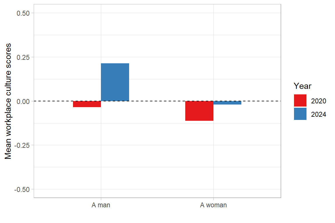
Click to see code producing the boxplot
# Boxplots for workplace culture scores by gender and year
df.geam20.24 |>
  select(year, gender, culture_mean) |>
  drop_na() |>
  ggplot(aes(x=gender, y=culture_mean, fill=as.factor(year))) +
    geom_boxplot(width=0.5) +
    geom_hline(yintercept = 0, color = "black", linetype = "dashed") +
    scale_fill_manual(values=cpal) +
    scale_y_continuous(limits = c(-2, 2)) +
    labs(x="", y="Mean workplace culture scores", fill="Year") +
    theme_light()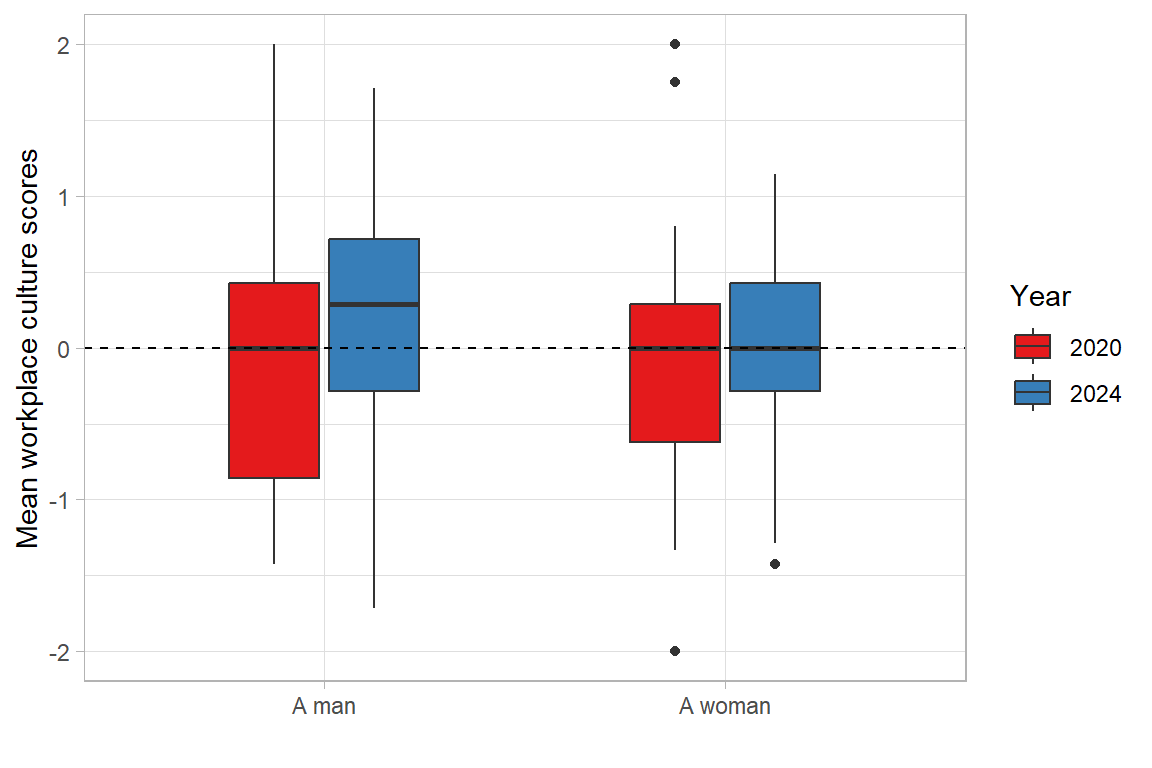
4.3.2.3 Regression analysis: workplace culture
Click to see code for base linear regression model 1 with year only
owcw_base <- lm(culture_mean ~ year, data = df.geam20.24)

owcw_base |>
  tbl_regression(intercept = T,
                 pvalue_fun = label_style_pvalue(digits = 3),) |>
modify_column_unhide(column = c(std.error, statistic)) | Characteristic | Beta | SE | Statistic | 95% CI | p-value |
|---|---|---|---|---|---|
| (Intercept) | -0.08 | 0.087 | -0.881 | -0.25, 0.09 | 0.379 |
| year | |||||
| 2020 | — | — | — | — | |
| 2024 | 0.11 | 0.102 | 1.10 | -0.09, 0.31 | 0.274 |
| Abbreviations: CI = Confidence Interval, SE = Standard Error | |||||
Click to see code for model 2
owcw_main <- lm(culture_mean ~ year + gender + manager + parent, data = df.geam20.24)

owcw_main |>
  tbl_regression(intercept = T,
                 pvalue_fun = label_style_pvalue(digits = 3),) |>
modify_column_unhide(column = c(std.error, statistic)) | Characteristic | Beta | SE | Statistic | 95% CI | p-value |
|---|---|---|---|---|---|
| (Intercept) | 0.01 | 0.117 | 0.122 | -0.22, 0.25 | 0.903 |
| year | |||||
| 2020 | — | — | — | — | |
| 2024 | 0.17 | 0.105 | 1.59 | -0.04, 0.37 | 0.113 |
| gender | |||||
| A man | — | — | — | — | |
| A woman | -0.16 | 0.095 | -1.71 | -0.35, 0.02 | 0.089 |
| manager | |||||
| No | — | — | — | — | |
| Yes | 0.14 | 0.137 | 1.01 | -0.13, 0.41 | 0.314 |
| parent | |||||
| Yes | — | — | — | — | |
| No | -0.02 | 0.094 | -0.207 | -0.21, 0.17 | 0.836 |
| Abbreviations: CI = Confidence Interval, SE = Standard Error | |||||
Click to see code for model 3
owcw_fit <- lm(culture_mean ~ gender*year + manager*year + parent*year, data=df.geam20.24)

owcw_fit |>
  tbl_regression(intercept = T,
                 pvalue_fun = label_style_pvalue(digits = 3),) |>
modify_column_unhide(column = c(std.error, statistic)) | Characteristic | Beta | SE | Statistic | 95% CI | p-value |
|---|---|---|---|---|---|
| (Intercept) | 0.11 | 0.173 | 0.631 | -0.23, 0.45 | 0.528 |
| gender | |||||
| A man | — | — | — | — | |
| A woman | -0.06 | 0.183 | -0.353 | -0.42, 0.30 | 0.724 |
| year | |||||
| 2020 | — | — | — | — | |
| 2024 | 0.06 | 0.200 | 0.287 | -0.34, 0.45 | 0.775 |
| manager | |||||
| No | — | — | — | — | |
| Yes | 0.19 | 0.262 | 0.734 | -0.32, 0.71 | 0.463 |
| parent | |||||
| Yes | — | — | — | — | |
| No | -0.27 | 0.186 | -1.46 | -0.64, 0.10 | 0.147 |
| gender * year | |||||
| A woman * 2024 | -0.14 | 0.214 | -0.660 | -0.56, 0.28 | 0.510 |
| year * manager | |||||
| 2024 * Yes | -0.10 | 0.308 | -0.331 | -0.71, 0.51 | 0.741 |
| year * parent | |||||
| 2024 * No | 0.34 | 0.216 | 1.59 | -0.08, 0.77 | 0.113 |
| Abbreviations: CI = Confidence Interval, SE = Standard Error | |||||
Click to see code for homoscedasticity test
bp_test <- car::ncvTest(owcw_fit)

bp_results <- data.frame(
  Test = "Breusch-Pagan",
  `Chi-square` = round(bp_test$ChiSquare, 2),
  Df = bp_test$Df,
  `p-value` = round(bp_test$p, 2)
)

bp_results | Test | Chi.square | Df | p.value |
|---|---|---|---|
| Breusch-Pagan | 2.78 | 1 | 0.1 |
The regression analysis in Table 4.11 indicates that factors such as timeframe, gender, managerial status, and parenthood are not statistically significant predictors of workplace culture perceptions.
4.3.3 Microaggressions (BIMA)
4.3.3.1 Preparation and transformation of data
df20 <- df.geam20 |>
  select(starts_with("BIMA001"))|>
  map_df(~ {if_else(.x == "Not applicable", NA, .x)}) |>  # replace "Not applicable" with NA
  map_df(~ {as.numeric(.x)-1}) |>
  mutate(micagg_mean = rowMeans(across(everything()), na.rm=T)) |>
  select(micagg_mean)

df24 <- df.geam24 |>
  select(starts_with("BIMA001"))|>
  map_df(~ {if_else(.x == "", NA, .x)}) |>  # English translation has empty string for Polish "Odmowa odpowiedzi" refuse to answer
  map_df(~ {as.numeric(.x)-1}) |>
  mutate(micagg_mean = rowMeans(across(everything()), na.rm=T)) |>
  select(micagg_mean)

df.geam20.24 <- bind_rows(df20, df24)  |>
bind_cols(df.geam20.24) 4.3.3.2 Mean analysis: microaggressions
Click to see code for producing BIMA mean scores
# Mean scores for microaggressions (BIMA)
df.geam20.24 |>
  select(year, gender, manager, parent, micagg_mean)|>
  drop_na()|>
  tbl_custom_summary(
    by = year,
    include = c(gender, manager, parent),
    stat_fns = everything() ~ function(data, ...){
       m <- mean(data$micagg_mean, na.rm = TRUE)
       tibble(mean_micagg_score = m)
    },
    statistic = everything() ~ "{mean_micagg_score}",
    digits = everything() ~ c(3),
    type = all_dichotomous() ~ "categorical",
    overall_row = T
) |>
  add_overall(last=T)|>
modify_spanning_header(all_stat_cols() ~ "**Mean microaggression**")| Characteristic |
Mean microaggression
|
||
|---|---|---|---|
| 2020 N = 591 |
2024 N = 1591 |
Overall N = 2181 |
|
| Overall | |||
| TRUE | 0.501 | 0.368 | 0.404 |
| FALSE | NA | NA | NA |
| gender | |||
| A man | 0.390 | 0.301 | 0.324 |
| A woman | 0.577 | 0.418 | 0.462 |
| manager | |||
| No | 0.478 | 0.363 | 0.393 |
| Yes | 0.626 | 0.402 | 0.469 |
| parent | |||
| Yes | 0.384 | 0.332 | 0.343 |
| No | 0.570 | 0.403 | 0.456 |
| 1 mean_micagg_score | |||
The data reveals that microaggressive behaviour was reported less frequently in 2024 than in 2020. The average value decreased from 0.50 in 2020 to 0.37 in 2024. Women, nonparents, and managers experienced microaggressions more often (in both 2020 and 2024). Although the mean is rather low for both years, it is worth noting that in 2024, the proportion of those who reported that they had experienced kinds of microaggression such as the dismissal or devaluation of their contribution or being ignored by colleagues at least ‘a little or rarely’ was considerable (over 40%).
Click to see the code for producing the barchart
# Barchart of mean microaggression scores
df.geam20.24 |>
  select(year, gender, micagg_mean) |>
  drop_na()|>
  group_by(year, gender) |>
  summarize(mean = mean(micagg_mean, na.rm=T)) |>
  ggplot(aes(x=gender, y=mean, fill=year)) +
    geom_bar(position="dodge", stat="identity", width=.5) +
    geom_hline(yintercept = 0, color = "black", linetype = "dashed") +
    scale_fill_manual(values=cpal) +
    scale_y_continuous(limits = c(-1, 1)) +
    labs(x="", y="Mean microaggresion scores", fill="Year") +
    theme_light()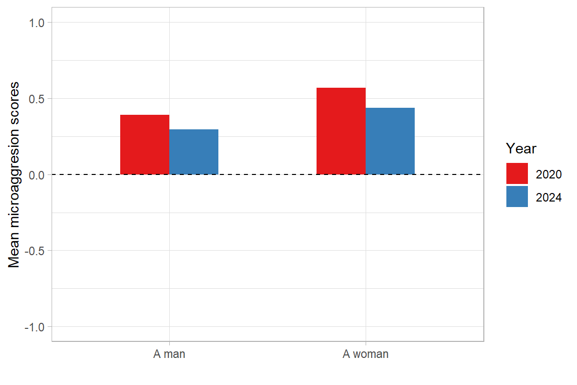
Click to see code producing the boxplot
# Boxplots for microagression scores by gender and year
df.geam20.24 |>
  select(year, gender, micagg_mean) |>
  drop_na() |>
  ggplot(aes(x=gender, y=micagg_mean, fill=as.factor(year))) +
    geom_boxplot(width=0.5) +
    geom_hline(yintercept = 0, color = "black", linetype = "dashed") +
    scale_fill_manual(values=cpal) +
    scale_y_continuous(limits = c(-0.2, 2.5)) +
    labs(x="", y="Mean microaggression scores", fill="Year") +
    theme_light()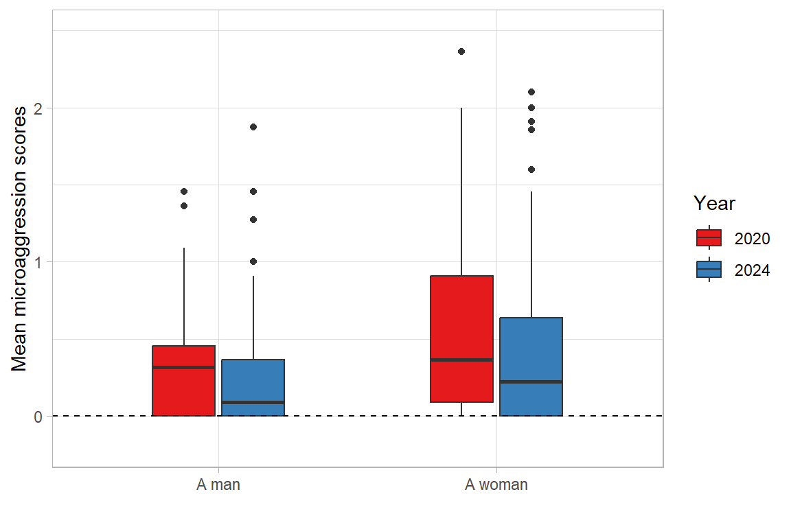
4.3.3.3 Regression analysis: microaggressions
Click to see code for model 1
micagg_base <- lm(micagg_mean ~ year, data = df.geam20.24)

micagg_base |>
  tbl_regression(intercept = T,
                 pvalue_fun = label_style_pvalue(digits = 3),) |>
modify_column_unhide(column = c(std.error, statistic)) | Characteristic | Beta | SE | Statistic | 95% CI | p-value |
|---|---|---|---|---|---|
| (Intercept) | 0.50 | 0.066 | 7.52 | 0.37, 0.63 | <0.001 |
| year | |||||
| 2020 | — | — | — | — | |
| 2024 | -0.09 | 0.077 | -1.21 | -0.24, 0.06 | 0.226 |
| Abbreviations: CI = Confidence Interval, SE = Standard Error | |||||
Click to see code for model 2
micagg_main <- lm(micagg_mean ~ year + gender + manager + parent, data = df.geam20.24)

micagg_main |>
  tbl_regression(intercept = T,
                 pvalue_fun = label_style_pvalue(digits = 3),) |>
modify_column_unhide(column = c(std.error, statistic)) | Characteristic | Beta | SE | Statistic | 95% CI | p-value |
|---|---|---|---|---|---|
| (Intercept) | 0.36 | 0.086 | 4.15 | 0.19, 0.53 | <0.001 |
| year | |||||
| 2020 | — | — | — | — | |
| 2024 | -0.12 | 0.076 | -1.55 | -0.27, 0.03 | 0.122 |
| gender | |||||
| A man | — | — | — | — | |
| A woman | 0.12 | 0.068 | 1.83 | -0.01, 0.26 | 0.069 |
| manager | |||||
| No | — | — | — | — | |
| Yes | 0.07 | 0.097 | 0.730 | -0.12, 0.26 | 0.466 |
| parent | |||||
| Yes | — | — | — | — | |
| No | 0.09 | 0.068 | 1.35 | -0.04, 0.23 | 0.178 |
| Abbreviations: CI = Confidence Interval, SE = Standard Error | |||||
Click to see code for model 3
micagg_fit <- lm(micagg_mean ~ gender*year + manager*year + parent*year, data=df.geam20.24)

micagg_fit |>
  tbl_regression(intercept = T,
                 pvalue_fun = label_style_pvalue(digits = 3),) |>
modify_column_unhide(column = c(std.error, statistic)) | Characteristic | Beta | SE | Statistic | 95% CI | p-value |
|---|---|---|---|---|---|
| (Intercept) | 0.27 | 0.130 | 2.12 | 0.02, 0.53 | 0.035 |
| gender | |||||
| A man | — | — | — | — | |
| A woman | 0.16 | 0.134 | 1.18 | -0.11, 0.42 | 0.238 |
| year | |||||
| 2020 | — | — | — | — | |
| 2024 | -0.01 | 0.148 | -0.049 | -0.30, 0.28 | 0.961 |
| manager | |||||
| No | — | — | — | — | |
| Yes | 0.13 | 0.183 | 0.706 | -0.23, 0.49 | 0.481 |
| parent | |||||
| Yes | — | — | — | — | |
| No | 0.18 | 0.134 | 1.34 | -0.09, 0.44 | 0.183 |
| gender * year | |||||
| A woman * 2024 | -0.05 | 0.156 | -0.304 | -0.35, 0.26 | 0.761 |
| year * manager | |||||
| 2024 * Yes | -0.08 | 0.217 | -0.390 | -0.51, 0.34 | 0.697 |
| year * parent | |||||
| 2024 * No | -0.12 | 0.156 | -0.755 | -0.43, 0.19 | 0.451 |
| Abbreviations: CI = Confidence Interval, SE = Standard Error | |||||
The results of the regression analysis as shown in Table 4.15 reveal no statistically significant effects of gender, year, nor being a manager or a parent on experiencing microaggressions. No statistically significant combined effects of gender and year, year and being a manager, nor year and being a parent on reporting microaggressions can be observed as shown in Table 4.16; the only statistically significant term (p<0.05) is an intercept.
Click to see code for homoscedasticity test
bp_test <- car::ncvTest(micagg_fit)

bp_results <- data.frame(
  Test = "Breusch-Pagan",
  `Chi-square` = round(bp_test$ChiSquare, 2),
  Df = bp_test$Df,
  `p-value` = round(bp_test$p, 2)
)

bp_results | Test | Chi.square | Df | p.value |
|---|---|---|---|
| Breusch-Pagan | 4.83 | 1 | 0.03 |
4.3.4 Gender equality (OCPER001)
4.3.4.1 Preparation and transformation of data
# merge OCPER001 items for year 2020
df20 <- df.geam20 |>
  select(starts_with("OCPER001"))|>
  map_df(~ {as.numeric(.x)-3}) |>
  mutate(genequ_mean = rowMeans(across(everything()), na.rm=T)) |>
  select(genequ_mean)

# merge OCPER001 items for year 2024
df24 <- df.geam24 |>
  select(starts_with("OCPER001"))|>
  map_df(~ {as.numeric(.x)-3}) |>
  mutate(genequ_mean = rowMeans(across(everything()), na.rm=T)) |>
  select(genequ_mean)

df.geam20.24 <- bind_rows(df20, df24)  |>
bind_cols(df.geam20.24) 4.3.4.2 Mean analysis: gender equality
Click to see code for producing OCPER001 mean scores table
# Calculate mean scores for OCPER001 by gender, manager, and parent status across years
df.geam20.24 |>
  select(year, gender, manager, parent, genequ_mean)|>
  drop_na()|>
  tbl_custom_summary(
    by = year,
    include = c(gender, manager, parent),
    stat_fns = everything() ~ function(data, ...){
       m <- mean(data$genequ_mean, na.rm = TRUE)
       tibble(mean_genequ_score = m)
    },
    statistic = everything() ~ "{mean_genequ_score}",
    digits = everything() ~ c(3),
    type = all_dichotomous() ~ "categorical",
    overall_row = T
) |>
  add_overall(last=T)|>
modify_spanning_header(all_stat_cols() ~ "**Mean gender equality**")| Characteristic |
Mean gender equality
|
||
|---|---|---|---|
| 2020 N = 621 |
2024 N = 1751 |
Overall N = 2371 |
|
| Overall | |||
| TRUE | 0.087 | 0.411 | 0.326 |
| FALSE | NA | NA | NA |
| gender | |||
| A man | 0.336 | 0.651 | 0.562 |
| A woman | -0.131 | 0.239 | 0.149 |
| manager | |||
| No | 0.061 | 0.404 | 0.315 |
| Yes | 0.244 | 0.460 | 0.399 |
| parent | |||
| Yes | 0.107 | 0.425 | 0.357 |
| No | 0.076 | 0.398 | 0.301 |
| 1 mean_genequ_score | |||
In 2020, the average value hovered around zero (0.09), which indicates that OPI PIB employees held no strong opinions on gender equality at the institute. In 2024, the mean had risen to 0.41, which suggests a slight shift towards agreement with the statements. When divided by gender, in the 2020 survey, women disagreed slightly with the notion of gender equality at the institute (−0.13); in 2024, however, they were somewhat more inclined to view it positively (0.24). Meanwhile, male perception of gender equality, which was already positive in 2020 (0.34), improved significantly, reaching 0.65 in 2024.
Click to see code producing the barchart
df.geam20.24 |>
  select(year, gender, genequ_mean) |>
  drop_na()|>
  group_by(year, gender) |>
  summarize(mean = mean(genequ_mean, na.rm=T)) |>
  ggplot(aes(x=gender, y=mean, fill=year)) +
  geom_bar(position="dodge", stat="identity", width=.5) +
  geom_hline(yintercept = 0, color = "black", linetype = "dashed") +
  scale_fill_manual(values=cpal) +
  scale_y_continuous(limits = c(-1, 1)) +
  labs(x="", y="Mean gender equality scores", fill="Year") +
  theme_light()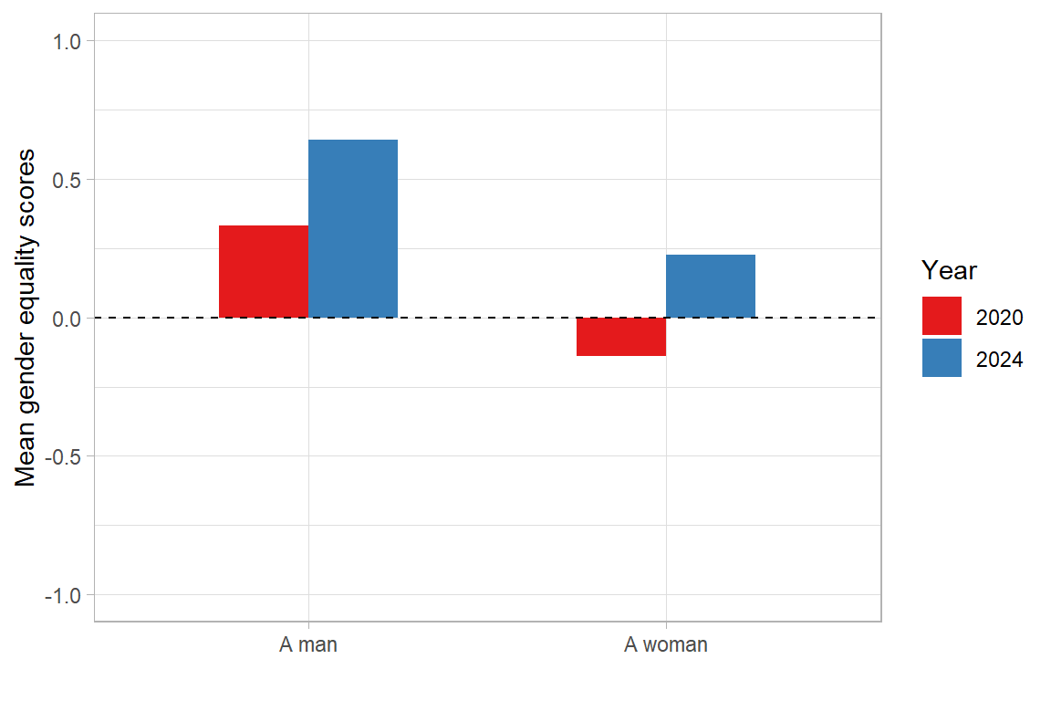
Click to see code producing the boxplot
df.geam20.24 |>
  select(year, gender, genequ_mean) |>
  drop_na() |>
  ggplot(aes(x=gender, y=genequ_mean, fill=as.factor(year))) +
  geom_boxplot(width=0.5) +
  geom_hline(yintercept = 0, color = "black", linetype = "dashed") +
  scale_fill_manual(values=cpal) +
  scale_y_continuous(limits = c(-2, 2)) +
  labs(x="", y="Mean gender equality scores", fill="Year") +
  theme_light()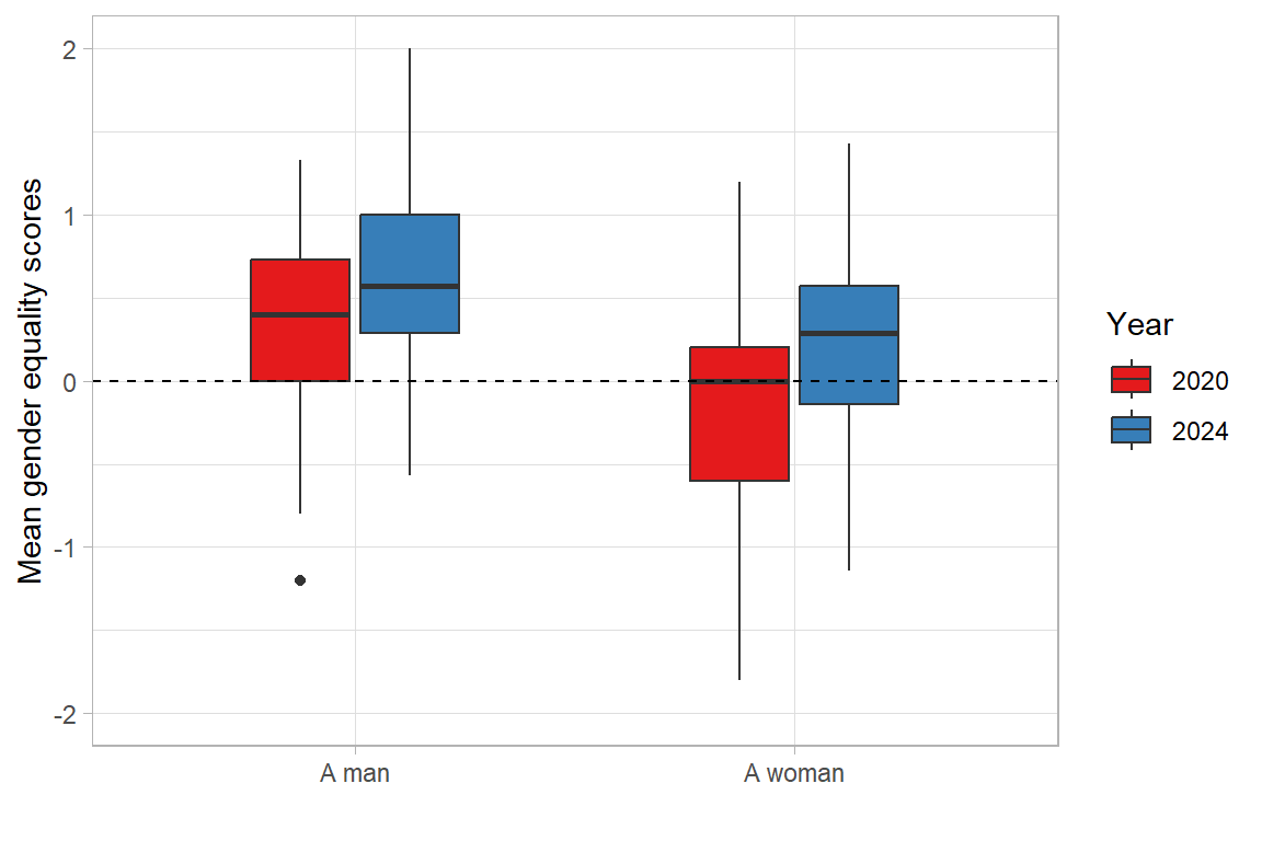
4.3.4.3 Regression analysis: gender equality
Click to see code for model 1
genequ_base <- lm(genequ_mean ~ year, data = df.geam20.24)

genequ_base |>
  tbl_regression(intercept = T,
                 pvalue_fun = label_style_pvalue(digits = 3),) |>
modify_column_unhide(column = c(std.error, statistic)) | Characteristic | Beta | SE | Statistic | 95% CI | p-value |
|---|---|---|---|---|---|
| (Intercept) | 0.08 | 0.077 | 1.09 | -0.07, 0.23 | 0.278 |
| year | |||||
| 2020 | — | — | — | — | |
| 2024 | 0.31 | 0.089 | 3.51 | 0.14, 0.49 | <0.001 |
| Abbreviations: CI = Confidence Interval, SE = Standard Error | |||||
Click to see code for model 2
genequ_main <- lm(genequ_mean ~ year + gender + manager + parent, data = df.geam20.24)

genequ_main |>
  tbl_regression(intercept = T,
                 pvalue_fun = label_style_pvalue(digits = 3),) |>
modify_column_unhide(column = c(std.error, statistic)) | Characteristic | Beta | SE | Statistic | 95% CI | p-value |
|---|---|---|---|---|---|
| (Intercept) | 0.29 | 0.097 | 2.95 | 0.10, 0.48 | 0.003 |
| year | |||||
| 2020 | — | — | — | — | |
| 2024 | 0.35 | 0.087 | 4.02 | 0.18, 0.52 | <0.001 |
| gender | |||||
| A man | — | — | — | — | |
| A woman | -0.43 | 0.077 | -5.60 | -0.58, -0.28 | <0.001 |
| manager | |||||
| No | — | — | — | — | |
| Yes | 0.12 | 0.111 | 1.09 | -0.10, 0.34 | 0.277 |
| parent | |||||
| Yes | — | — | — | — | |
| No | 0.02 | 0.077 | 0.263 | -0.13, 0.17 | 0.793 |
| Abbreviations: CI = Confidence Interval, SE = Standard Error | |||||
Click to see code for model 3
genequ_fit <- lm(genequ_mean ~ gender*year + manager*year + parent*year, data=df.geam20.24)

genequ_fit |>
  tbl_regression(intercept = T,
                 pvalue_fun = label_style_pvalue(digits = 3),) |>
modify_column_unhide(column = c(std.error, statistic)) | Characteristic | Beta | SE | Statistic | 95% CI | p-value |
|---|---|---|---|---|---|
| (Intercept) | 0.28 | 0.145 | 1.94 | 0.00, 0.57 | 0.054 |
| gender | |||||
| A man | — | — | — | — | |
| A woman | -0.52 | 0.153 | -3.40 | -0.82, -0.22 | <0.001 |
| year | |||||
| 2020 | — | — | — | — | |
| 2024 | 0.36 | 0.167 | 2.13 | 0.03, 0.68 | 0.034 |
| manager | |||||
| No | — | — | — | — | |
| Yes | 0.34 | 0.219 | 1.57 | -0.09, 0.78 | 0.117 |
| parent | |||||
| Yes | — | — | — | — | |
| No | 0.05 | 0.157 | 0.335 | -0.26, 0.36 | 0.738 |
| gender * year | |||||
| A woman * 2024 | 0.11 | 0.178 | 0.605 | -0.24, 0.46 | 0.546 |
| year * manager | |||||
| 2024 * Yes | -0.30 | 0.256 | -1.16 | -0.80, 0.21 | 0.247 |
| year * parent | |||||
| 2024 * No | -0.04 | 0.181 | -0.196 | -0.39, 0.32 | 0.844 |
| Abbreviations: CI = Confidence Interval, SE = Standard Error | |||||
Click to see code for homoscedasticity test
bp_test <- car::ncvTest(genequ_fit)

bp_results <- data.frame(
  Test = "Breusch-Pagan",
  `Chi-square` = round(bp_test$ChiSquare, 2),
  Df = bp_test$Df,
  `p-value` = round(bp_test$p, 2)
)

bp_results | Test | Chi.square | Df | p.value |
|---|---|---|---|
| Breusch-Pagan | 0.64 | 1 | 0.42 |
The regression analysis indicates significant effects (p < 0.05) of gender and year on the responses. Women rated the situation worse than men—although in 2024, ratings increased significantly compared to 2020. Neither holding a managerial position nor being a parent had any significant impact on the responses. No significant interaction effects between variables over the years were found, meaning that the differences between 2020 and 2024 were similar across different groups.
In summary, the perception of equality at OPI PIB improved significantly in 2024 compared to 2020. However, men were considerably more likely than women to perceive OPI PIB as an organisation that promotes equality. Managerial status or parenthood are not significant for the perception of equality.
4.3.5 Gender equality: resources or responsibilities (OCPER003)
4.3.5.1 Preparation and transformation of data
# merge selected OCPER003 items for 2020
df20 <- df.geam20 |>
  select(num_range("OCPER003_SQ", c(3,4,6,7,9,10,11,14,16,18,19), width=3)) |> # select sub-questions 3, 4, ...
  map_df(~ {if_else(.x == "Not applicable", NA, .x)}) |>  # replace "Not applicable" with NA
  map_df(~ {as.numeric(.x)-3}) |>                         # convert factor to numeric and center on 0
  mutate(ocper3_mean = rowMeans(across(everything()), na.rm=T)) |>
  select(ocper3_mean)

# merge selected OCPER003 items for 2024
df24 <- df.geam24 |>
  select(num_range("OCPER003.SQ", c(1,2,4:8, 10:13), width=3)) |>
  map_df(~ {if_else(.x == "No opinion", NA, .x)}) |>
  map_df(~ {as.numeric(.x)-3}) |>
  mutate(ocper3_mean = rowMeans(across(everything()), na.rm=T)) |>
  select(ocper3_mean)

df.geam20.24 <- bind_rows(df20, df24)  |>
bind_cols(df.geam20.24) 4.3.5.2 Mean analysis: resources or responsibilities
Click to see code for producing OCPER003 mean scores table
df.geam20.24 |>
  select(year, gender, manager, parent, ocper3_mean)|>
  drop_na()|>
  tbl_custom_summary(
    by = year,
    include = c(gender, manager, parent),
    stat_fns = everything() ~ function(data, ...){
       m <- mean(data$ocper3_mean, na.rm = TRUE)
       tibble(mean_ocper3_score = m)
    },
    statistic = everything() ~ "{mean_ocper3_score}",
    digits = everything() ~ c(3),
    type = all_dichotomous() ~ "categorical",
    overall_row = T
) |>
  add_overall(last=T)|>
modify_spanning_header(all_stat_cols() ~ "**Mean resources**")| Characteristic |
Mean resources
|
||
|---|---|---|---|
| 2020 N = 651 |
2024 N = 1591 |
Overall N = 2241 |
|
| Overall | |||
| TRUE | 0.152 | 0.251 | 0.222 |
| FALSE | NA | NA | NA |
| gender | |||
| A man | -0.116 | -0.093 | -0.100 |
| A woman | 0.368 | 0.488 | 0.455 |
| manager | |||
| No | 0.127 | 0.247 | 0.213 |
| Yes | 0.289 | 0.275 | 0.280 |
| parent | |||
| Yes | 0.082 | 0.218 | 0.186 |
| No | 0.196 | 0.283 | 0.254 |
| 1 mean_ocper3_score | |||
The data indicates a small but persistent trend that the resources and responsibilities mentioned in the question are more often assigned to men than to women (with an average value close to 0.15 in 2020 and 0.25 in 2024). In 2024 women reported higher average values than men (0.49), which suggests that they are more likely to perceive inequality to the disadvantage of women. Men perceive that resources are assigned to women slightly more often, but the difference is minimal. Between 2020 and 2024, no significant changes could be observed in the perception of gender equality in resource allocation.
Click to see code producing the barchart
df.geam20.24 |>
  select(year, gender, ocper3_mean) |>
  drop_na()|>
  group_by(year, gender) |>
  summarize(mean = mean(ocper3_mean, na.rm=T)) |>
  ggplot(aes(x=gender, y=mean, fill=year)) +
    geom_bar(position="dodge", stat="identity", width=.5) +
    geom_hline(yintercept = 0, color = "black", linetype = "dashed") +
    scale_fill_manual(values=cpal) +
    scale_y_continuous(limits = c(-1, 1)) +
    labs(x="", y="Mean resources or responsibilities scores", fill="Year") +
    theme_light()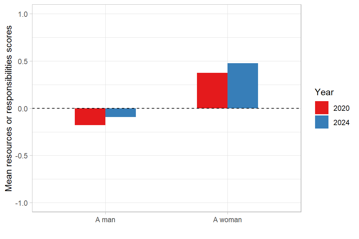
Click to see code producing the boxplot
df.geam20.24 |>
  select(year, gender, ocper3_mean) |>
  drop_na() |>
  ggplot(aes(x=gender, y=ocper3_mean, fill=as.factor(year))) +
  geom_boxplot(width=0.5) +
  geom_hline(yintercept = 0, color = "black", linetype = "dashed") +
  scale_fill_manual(values=cpal) +
  scale_y_continuous(limits = c(-2, 2)) +
  labs(x="", y="Mean resources or responsibilities scores", fill="Year") +
  theme_light()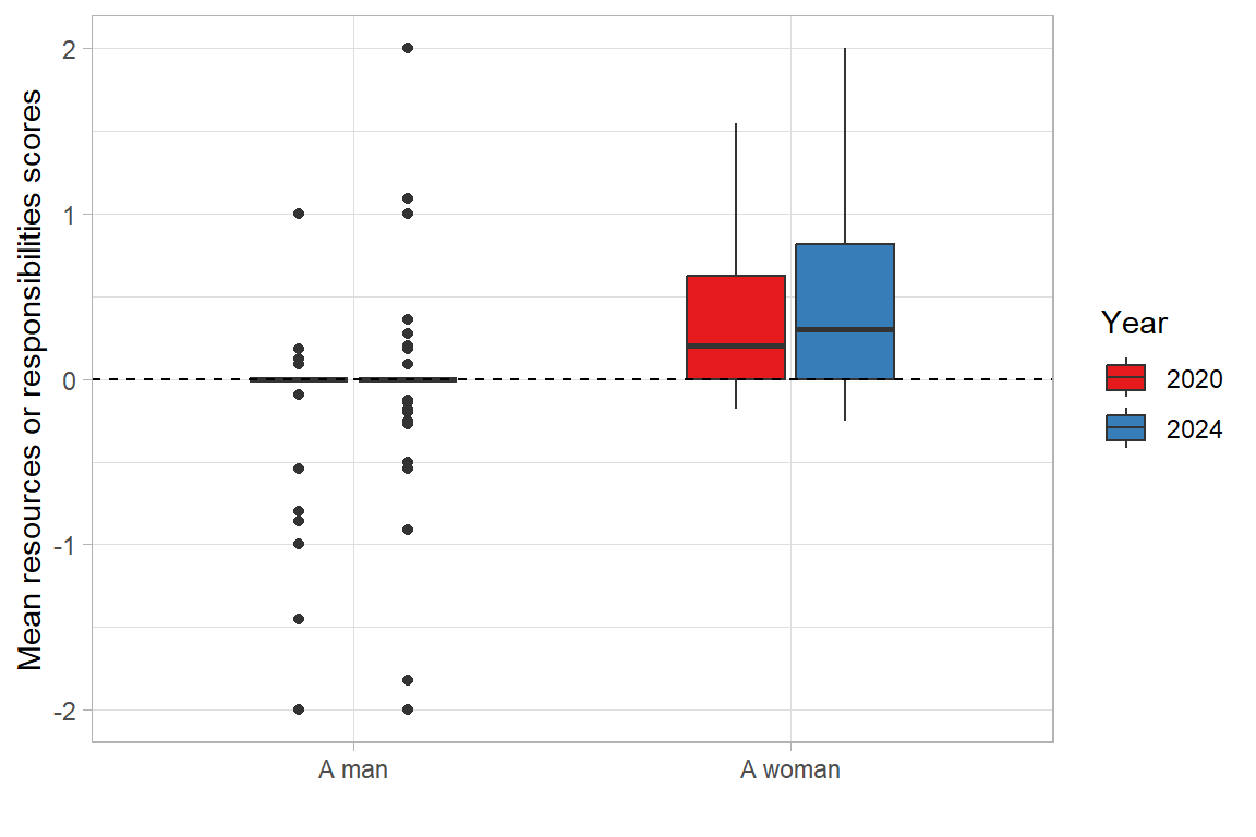
4.3.5.3 Regression analysis: resources or responsibilities
Click to see code for model 1
ocper3_base <- lm(ocper3_mean ~ year, data = df.geam20.24)

ocper3_base |>
  tbl_regression(intercept = T,
                 pvalue_fun = label_style_pvalue(digits = 3),) |>
modify_column_unhide(column = c(std.error, statistic)) | Characteristic | Beta | SE | Statistic | 95% CI | p-value |
|---|---|---|---|---|---|
| (Intercept) | 0.10 | 0.076 | 1.34 | -0.05, 0.25 | 0.183 |
| year | |||||
| 2020 | — | — | — | — | |
| 2024 | 0.14 | 0.089 | 1.60 | -0.03, 0.32 | 0.111 |
| Abbreviations: CI = Confidence Interval, SE = Standard Error | |||||
Click to see code for model 2
ocper3_main <- lm(ocper3_mean ~ year + gender + manager + parent, data = df.geam20.24)

ocper3_main |>
  tbl_regression(intercept = T,
                 pvalue_fun = label_style_pvalue(digits = 3),) |>
modify_column_unhide(column = c(std.error, statistic)) | Characteristic | Beta | SE | Statistic | 95% CI | p-value |
|---|---|---|---|---|---|
| (Intercept) | -0.17 | 0.089 | -1.93 | -0.35, 0.00 | 0.055 |
| year | |||||
| 2020 | — | — | — | — | |
| 2024 | 0.08 | 0.079 | 1.03 | -0.08, 0.24 | 0.306 |
| gender | |||||
| A man | — | — | — | — | |
| A woman | 0.55 | 0.073 | 7.52 | 0.41, 0.69 | <0.001 |
| manager | |||||
| No | — | — | — | — | |
| Yes | 0.05 | 0.104 | 0.492 | -0.15, 0.26 | 0.623 |
| parent | |||||
| Yes | — | — | — | — | |
| No | 0.02 | 0.073 | 0.270 | -0.12, 0.16 | 0.788 |
| Abbreviations: CI = Confidence Interval, SE = Standard Error | |||||
Click to see code for model 3
ocper3_fit <- lm(ocper3_mean ~ gender*year + manager*year + parent*year, data=df.geam20.24)

ocper3_fit |>
  tbl_regression(intercept = T,
                 pvalue_fun = label_style_pvalue(digits = 3),) |>
modify_column_unhide(column = c(std.error, statistic)) | Characteristic | Beta | SE | Statistic | 95% CI | p-value |
|---|---|---|---|---|---|
| (Intercept) | -0.17 | 0.130 | -1.31 | -0.43, 0.09 | 0.191 |
| gender | |||||
| A man | — | — | — | — | |
| A woman | 0.47 | 0.138 | 3.43 | 0.20, 0.74 | <0.001 |
| year | |||||
| 2020 | — | — | — | — | |
| 2024 | 0.07 | 0.152 | 0.466 | -0.23, 0.37 | 0.642 |
| manager | |||||
| No | — | — | — | — | |
| Yes | 0.04 | 0.191 | 0.195 | -0.34, 0.41 | 0.846 |
| parent | |||||
| Yes | — | — | — | — | |
| No | 0.09 | 0.138 | 0.650 | -0.18, 0.36 | 0.516 |
| gender * year | |||||
| A woman * 2024 | 0.11 | 0.163 | 0.690 | -0.21, 0.43 | 0.491 |
| year * manager | |||||
| 2024 * Yes | 0.04 | 0.229 | 0.157 | -0.41, 0.49 | 0.876 |
| year * parent | |||||
| 2024 * No | -0.10 | 0.163 | -0.615 | -0.42, 0.22 | 0.539 |
| Abbreviations: CI = Confidence Interval, SE = Standard Error | |||||
Click to see code for homoscedasticity test
bp_test <- car::ncvTest(ocper3_fit)

bp_results <- data.frame(
  Test = "Breusch-Pagan",
  `Chi-square` = round(bp_test$ChiSquare, 2),
  Df = bp_test$Df,
  `p-value` = round(bp_test$p, 2)
)

bp_results | Test | Chi.square | Df | p.value |
|---|---|---|---|
| Breusch-Pagan | 0.7 | 1 | 0.4 |
Regression analysis confirms that gender is statistically significant factor in the allocation of resources and responsibilities: the coefficient for the gender variable is 0.47 and is statistically significant (p < 0.05). Considering the time frame, the situation has not changed significantly compared to 2020 (p > 0.05). Being a manager or a parent is also not a significant predictor (p > 0.05), which means their influence on resource allocation is not pronounced. In conclusion, gender is a key factor: women are more likely to perceive that resources are allocated to men, and this situation has remained consistent between 2020 and 2024.
4.4 Limitations
While this regression model provides valuable insights into potential changes in the factors influencing work culture (OCWC), masculinity contest culture (MCC), respondents’ experiences of microaggressions at work (BIMA), overall perceptions of equality practices at the institute (OCPER001), and the redistribution of resources and responsibilities (OCPER003), several limitations should be considered:
4.4.1 Cross-sectional nature of the data
The study relies on cross-sectional data, meaning that different individuals were observed in 2020 and 2024, rather than tracking the same respondents over time. This limits the ability to observe individual changes in perceptions, experiences, and attitudes. For example, the individuals who responded in 2020 may have had different opinions or work experiences compared to those who responded in 2024. Without following the same individuals over time, it is difficult to determine if the change observed in responses reflects a real shift in workplace conditions or if it is simply due to differences in the respondents’ characteristics, such as changes in personnel or new individuals with different attitudes. As a result, temporal shifts in the dependent variables may not be fully captured, and potential unobserved heterogeneity could bias the estimates.
Potential Solution: While obtaining longitudinal data is challenging due to strict data protection policies, alternative approaches could be used. For example, synthetic cohort methods could be employed, where groups of individuals with similar characteristics (such as gender, role, or research area) in 2020 and 2024 are compared. This approach allows for approximating longitudinal analysis by creating pseudo-panels based on shared characteristics.
4.4.2 Potential omitted variable bias
Although the model incorporates key predictors, such as gender, managerial role, and parental status, there may be other important factors influencing the dependent variables, such as academic field, department dynamics, or institutional policies. The exclusion of these factors could result in omitted variable bias, leading to inaccurate or biased estimates.
Potential Solution: Future studies could include additional control variables related to institutional factors, such as departmental culture or academic field, to reduce omitted variable bias. While data protection concerns limit access to detailed personal or departmental information, collaborating with institutional leadership or using publicly available departmental characteristics may help mitigate this issue.
4.4.3 Assumption of homogeneous effects
The model assumes that the effects of gender, managerial role, and other variables are uniform across all respondents. However, the influence of these variables may differ based on factors such as research discipline, tenure status, or other institutional roles. Differences in career trajectories, department cultures, or personal experiences could lead to heterogeneous effects, which may not be fully captured by the model.
Potential Solution: Future research could explore these variations by conducting subgroup analyses to examine whether the effects of predictors differ by research discipline, career stage, or department. Additionally, incorporating interaction terms for specific demographic or institutional characteristics could allow for a more nuanced understanding of these variations.
Despite these limitations, the model offers an important framework for understanding changes in work culture, perceptions of equality, and experiences of microaggressions at the institute over time. Future research could address these limitations by using techniques such as synthetic cohorts, incorporating additional control variables, incorporating retrospective questions, and conducting subgroup analyses to enhance the robustness and validity of the findings. Although longitudinal data may not be feasible due to data protection constraints, these alternative approaches could provide valuable insights into the dynamics of workplace perceptions and experiences.
As an additional option, qualitative data such as interviews or focus groups could be employed alongside the survey data to capture more nuanced changes in perceptions and experiences. This could provide a deeper understanding of the trends observed between 2020 and 2024 and give context to the quantitative findings.
4.5 Conclusions
Changes in perceptions of workplace culture indicate positive effects from institutional actions, particularly with regard to perceived equality. Although these changes are noticeable, efforts to improve the perception of equality must continue. Further studies should focus on analysing the impact of the policies implemented after 2020 to determine whether these positive changes form part of a broader trend. Our findings also suggest that although changes in the perception of equality at OPI PIB are beginning to yield positive effects, this process must continue. Although changes are being noticed, they are not yet translating into real changes in access to valuable resources; perhaps more time is needed for this to happen. It is therefore crucial that the results in the coming years be monitored to assess whether the changes observed in 2024 are the result of transitional actions or part of long-term trends.
Despite progress in gender equality, differences persist in how men and women perceive equality. Although gender was statistically insignificant for perceptions of workplace culture, masculinity contest culture, and the reporting of microaggressions, a more detailed analyses would enable us to understand why male respondents, on average, have better perceptions of workplace culture and stronger agreement that their work environment does not support masculine norms, as well as why women report microaggressions more frequently than men do.
Similarly, although statistically insignificant, differences can be observed in the perceptions of individuals in different job roles. A key area for further analysis is the influence of managerial roles on organisational perceptions, as the results suggest that men, particularly those who occupy managerial positions, view the situation more neutrally than women or nonmanagers do.
When analysing changes in the frequencies of certain phenomena (such as microaggressions), it must be remembered that values above zero, although lower than in the previous surveys, still indicate the presence of undesirable behaviours.
Analysis of the results from 2020 and 2024 requires attention to be paid to subtle methodological differences, such as changes in question wording or reference periods. While these adjustments were made to simplify the answering process, they might affect the comparability of the results. The readers of the manual should focus on the consistency of questions and be conscious that more nuanced results could be achieved when considering the sub-dimensions within the scales.
Future studies might involve conducting more detailed analyses of changes in the perception of equality, focusing on different professional and family groups (e.g., mothers, nonmanagerial employees). Conducting more in-depth analyses with multifaceted tools could provide a fuller understanding of the situation at OPI PIB.
It is also worth exploring the impact of hybrid/remote work models on organisational culture to investigate whether the shift to remote work has mitigated certain issues (such as microaggressions) temporarily, and whether a return to in-person work might reverse those effects. Understanding the long-term sustainability of the changes will be crucial in the shaping of future policies.
Acknowledgements
The authors are gratefull for the extremely helpful commments provided by Dalia Argudo on the possible limiations of this study.
4.6 Appendix
4.6.1 Working culture (OCWC)
| Feature | 2020 | 2024 |
|---|---|---|
| Coding | ||
| -2: strongly disagree; -1: disagree; 0: no opinion; 1: agree; 2: strongly agree | ✓ | ✓ |
| Items | ||
| Workload is allocated in a fair and transparent manner | ✓ | ✓ |
| I am encouraged to undertake activities that contribute to my career development | ✓ | ✓ |
| I have a formally assigned mentor who I see regularly | ✓ | ✓ |
| I have the opportunity to serve on important institution committees | ✓ | ✓ |
| My institution values my external professional activities | ✓ | ✓ |
| Senior staff are inaccessible to me* | ✓ | |
| Senior management (directors) is accessible to me | ✓ | |
| I have an unsupportive manager* | ✓ | |
| I have a supportive line manager | ✓ | |
| Cronbach’s Alpha | 0.72 | 0.78 |
4.6.2 Masculinity contest culture (MCC)
| Feature | 2020 | 2024 |
|---|---|---|
| Coding | ||
| -2: not at all true; -1: somewhat untrue; 0: neither true nor untrue; 1: somewhat true; 2: entirely true | ✓ | ✓ |
| Items | ||
| Admitting you don’t know the answer looks weak | ✓ | ✓ |
| Expressing any emotion other than anger or pride is seen as weak | ✓ | ✓ |
| It’s important to be in good physical shape to be respected | ✓ | ✓ |
| People who are physically smaller have to work harder to get respect | ✓ | ✓ |
| To succeed you can’t let family interfere with work | ✓ | ✓ |
| Taking days off is frowned upon | ✓ | ✓ |
| You’re either ‘in’ or you’re ‘out,’ and once you’re out, you’re out | ✓ | ✓ |
| If you don’t stand up for yourself, people will step on you | ✓ | ✓ |
| Cronbach’s Alpha | 0.91 | 0.85 |
4.6.3 Microaggressions (BIMA001)
| Feature | 2020 | 2024 |
|---|---|---|
| Coding | ||
| 0: never; 1: a little or rarely; 2: sometimes; 3: often or frequently | ✓ | ✓ |
| Items | ||
| I am often mistaken for being a lower-status worker | ✓ | ✓ |
| I am treated like a second-class citizen | ✓ | ✓ |
| I feel that the people I work with do not pay attention to me or do not see my opinions as relevant | ✓ | ✓ |
| My contributions are dismissed or devalued | ✓ | ✓ |
| Colleagues have prejudices about my intelligence and abilities | ✓ | ✓ |
| Others assume that I will act aggressively or are scared of me | ✓ | ✓ |
| Colleagues ask me where I am from, suggesting that I do not belong | ✓ | ✓ |
| I notice that there are few role models at OPI PIB with a similar background to my own | ✓ | ✓ |
| Others hint that I should work harder to prove that I am not like other people from my background | ✓ | ✓ |
| Others suggest that people from my background get unfair benefits | ✓ | ✓ |
| Some colleagues deny that people from my background face extra obstacles | ✓ | ✓ |
| Cronbach’s Alpha | 0.86 | 0.87 |
4.6.4 Gender equality (OCPER001)
| Feature | 2020 | 2024 |
|---|---|---|
| Coding | ||
| -2: strongly disagree; -1: disagree; 0: no opinion; 1: agree; 2: strongly agree | ✓ | ✓ |
| Items | ||
| In general, men and women are equally represented in my institution | ✓ | ✓ |
| In general, men and women are treated equally in my institution | ✓ | ✓ |
| My institution is committed to promoting gender equality | ✓ | ✓ |
| Myself and colleagues know who to go to for gender equality concerns | ✓ | ✓ |
| My institution is responsive to gender equality concerns | ✓ | ✓ |
| Cronbach’s Alpha | 0.70 | 0.76 |
4.6.5 Gender equality: resources or responsibilities (OCPER003)
| Feature | 2020 | 2024 |
|---|---|---|
| Coding | ||
| -2: mainly allocated to women; -1: often allocated to women; 0: no difference; 1: often allocated to men; 2: mainly allocated to men | ✓ | ✓ |
| Items | ||
| The receipt of mentoring and/or guidance in making career decisions | ✓ | ✓ |
| Representation in senior positions | ✓ | ✓ |
| Positive attention from senior management | ✓ | ✓ |
| Access to informal circles of influence | ✓ | ✓ |
| Recruitment and selection of new staff | ✓ | ✓ |
| Promotion decisions | ✓ | ✓ |
| Formal training and career development opportunities | ✓ | ✓ |
| Invitations or opportunities to attend conferences, lectures, etc. | ✓ | ✓ |
| Recognition of intellectual contributions | ✓ | ✓ |
| Funds and monetary resources | ✓ | ✓ |
| Awards and recognition of excellence | ✓ | ✓ |
| Cronbach’s Alpha | 0.94 | 0.94 |