Click to see code for making gender binary
df.geam02 <- df.geam02 |>
mutate(SDEM004.bin = case_when(
SDEM004 == "Prefer not to say" ~ NA,
SDEM004 == "Non-binary" ~ NA,
SDEM004 == "Other" ~ NA,
.default = SDEM004
))This chapter provides a comprehensive overview of gender gap identification using GEAM questionnaire data, employing bivariate analysis techniques such as Chi-squared tests, Student’s t-tests, and analysis of variance (ANOVA). Key aspects including working conditions, work-life balance, and organisational culture are explored, offering practical tools for analysing and understanding gender inequalities in various contexts.
Gender gaps, Bivariate analysis, Statistical significance, chi-square, t-test, ANOVA, Contingency table
The GEAM questionnaire collects information on various aspects of working life, including work-life balance, job satisfaction, organisational culture, and other key factors. Detecting gender gaps with GEAM data involves analysing how responses differ between genders across the dimensions assessed.
Different statistical techniques are used depending on the nature of the variables and the study objectives. Chapter 2 introduced statistical methods such as frequency distributions, percentages, and contingency tables, which provide an initial overview of the data and help identify potential patterns or differences between genders.
This chapter takes the analysis further by assessing whether the observed gender differences are statistically significant; therefore, they are unlikely to be due to chance and instead reflect real disparities.
We begin by applying bivariate analysis techniques before progressing to more complex multivariate analysis techniques in later chapters. The choice between these approaches depends on the complexity of the analysis required, the type of data available, and the specific research questions. Each method has its advantages and limitations.
In the following sections, we analyse gender gaps across a selection of GEAM variables to demonstrate the different statistical techniques to be applied according to the type of variables used (categorical or continuous). For a more thematic oriented analysis of working conditions, working climate or bullying and harassment, see Part II of this handbook.
Three real databases from three organisations are used. These databases are identified as df.geam01, df.geam02, and df.geam03. The main difference between the databases is the adaptation of some variables (questions) to the respective organisational context, without significantly modifying the statistical analysis of this chapter.
The GEAM questionnaire contains many questions that yield categorical variables such as gender, job positions, type of contract among others. A categorical variable is a variable that represents categories or groups, rather than numerical values. For example SDEM004 (Gender) is a categorical variable where answers fall into 4 possible groups (see also Section 2.1.1): “A man”, “A women”, “Non-binary” or “Prefer to self-identify as…”.
Crossing all answer options by two categorical variables produces a contingency table.
To identify potential gender gaps, we will begin by assessing whether gender influences the distribution of roles within the organisation. To do so, we will focus on determining whether there is a statistically significant relationship between gender and job positions.
To explore this relationship, it is essential to first conduct a visual analysis that allows for a clear comparison of the distribution of gender across different job roles.
A 100% stacked bar chart is a suitable tool for this purpose, as it facilitates the visualisation of gender proportions within each type of position. By stacking the bars to 100%, we can directly observe the relative representation of men and women within each job category, irrespective of the total number of employees.
This type of chart helps identify potential gender gaps in the distribution of roles, highlighting whether one gender is overrepresented or underrepresented in specific areas of the organisation, which is crucial for understanding workplace equity and diversity dynamics.
The graph uses the binary gender variable SDEM004.bin and remove all NAs from both the gender as well as job position.
Since these stacked barchars between two categorical variables are quite frequent, we have created a custom function crosstab_plot() to generate the plots on the fly with different variables. It saves repeating the same lines of code for each plot.
#  Calculate gender proportions
df.prop.01 <- df.geam01 |>
  filter(!is.na(WCJC001) & !is.na(SDEM004.bin)) |>
  group_by(SDEM004.bin, WCJC001) |>
  summarise(n = n(), .groups = "drop") |>
  group_by(SDEM004.bin) |>
  mutate(
    prop = n / sum(n),
    label = ifelse(prop > 0.03, paste0(n, " (", scales::percent(prop, accuracy = 1), ")"), "")
  )

# define colors
cpal <- RColorBrewer::brewer.pal(5, "Set1")

# create stacked bar chart
p1 <- df.prop.01 |>
  ggplot(aes(x = SDEM004.bin, y = prop, fill = WCJC001)) +
    geom_col(width = 0.8, position = "stack") +
    geom_text(aes(label = label),
            position = position_stack(vjust = 0.5),
            color = "white", size = 3.5, lineheight = 0.9) +
    scale_fill_manual(values = cpal) +
    scale_y_continuous(labels = percent_format()) +
    labs(x = "", y = "Proportion", fill = "Job Position") +
    theme_light()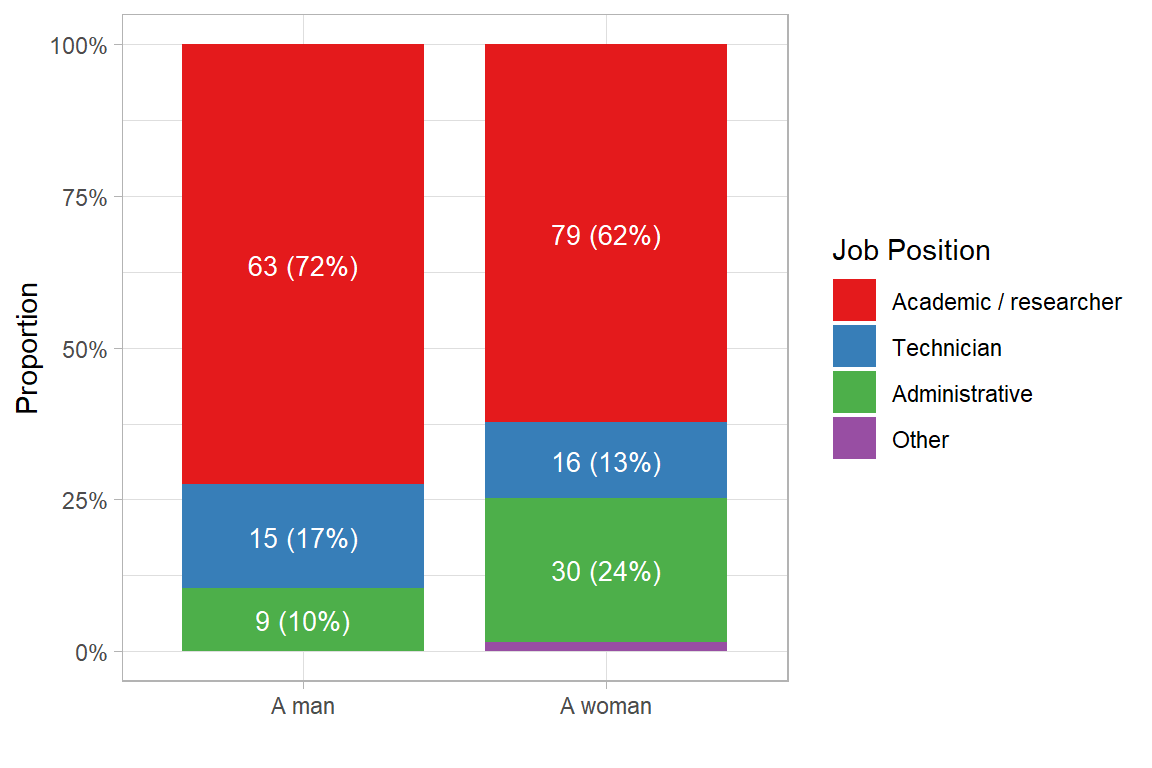
Figure 3.1 shows the relative distribution of jobs by gender, highlighting differentiated patterns between men and women. We observe that 72% of men hold academic or research positions, compared to 62% of women in the same category. On the other hand, women are overrepresented in administrative roles, with 24% compared to 10% of men. These differences suggest the existence of occupational segregation by gender, which may reflect structural dynamics of inequality within the organisation. The categories of technician and other positions show smaller discrepancies, though they still contribute to the overall pattern of unequal distribution. This trend requires further exploration through statistical tests to determine the significance of the observed differences.
In addition to the bar chart, a contingency table will also be used to display the observed frequencies and identify patterns between the variables. In order to generate contingency tables, we use the gtsummary package.
df.geam01 |>
  filter(!is.na(WCJC001) & !is.na(SDEM004.bin)) |>
  tbl_cross(
    row = SDEM004.bin,
    col = WCJC001
  ) |>
  bold_labels()
What is your current professional category at your organisation?
|
Total | ||||
|---|---|---|---|---|---|
| Academic / researcher | Technician | Administrative | Other | ||
| Are you | |||||
| A man | 63 | 15 | 9 | 0 | 87 |
| Non-binary | 0 | 0 | 0 | 0 | 0 |
| A woman | 79 | 16 | 30 | 2 | 127 |
| Prefer not to say | 0 | 0 | 0 | 0 | 0 |
| Other | 0 | 0 | 0 | 0 | 0 |
| Total | 142 | 31 | 39 | 2 | 214 |
Like the graph, the Table 3.1 crosstab shows the observed frequencies at the intersection of the variables of interest. This table helps us visualize categories or levels with very small or zero values. for the variables of interest.
One cell has a value of 0, corresponding to the intersection of the Other and A man categories. Besides filtering out missing values (NAs), it is crucial to exclude categories with no observations before testing for independence between qualitative variables.
Next, we create a subsample by dropping empty levels for each factor variable (NAs) from SDEM004.bin and WCJC001 and excluding the Other category from WCJC001.
Excluding empty categories is essential, as the Chi-square test requires at least 5 observations per cell for valid results.
df.sub.01 <- df.geam01 |>
  filter(!is.na(WCJC001) & WCJC001 != "Other" & !is.na(SDEM004.bin)) |>
  transmute(
    Jobpos = fct_drop(WCJC001),
    Gender = fct_drop(SDEM004.bin)
)Since both gender and job position are categorical variables, we will apply association tests to determine (Chi-squared, Cramér’s V, Fisher) whether the observed differences are statistically significant, indicating a relationship between the variables, or whether they are independent.
# custom function to calculate different test statistics: chi-square, cramer, fisher
statsnote <- crosstab_stats(df.sub.01, "Gender", "Jobpos")

# create the contingency table
df.sub.01 |>
  tbl_cross(
    row = Gender,
    col = Jobpos,
    percent = c("row"),
  ) |>
  bold_labels() |>
  modify_footnote_header(
    footnote = statsnote[[1]],
    columns = last_col(),
    replace=F
  )
What is your current professional category at your organisation?
|
Total1 | |||
|---|---|---|---|---|
| Academic / researcher | Technician | Administrative | ||
| Are you | ||||
| A man | 63 (72%) | 15 (17%) | 9 (10%) | 87 (100%) |
| A woman | 79 (63%) | 16 (13%) | 30 (24%) | 125 (100%) |
| Total | 142 (67%) | 31 (15%) | 39 (18%) | 212 (100%) |
| 1 Chi-squared = 6.542 | p-value = 0.038 | df = 2 | Cramér’s V = 0.176 | Fisher’s p = 0.0332 | ||||
Table 3.2 displays the absolute frequencies, the corresponding row percentages for each category, and several statistical test.
The result of the chi-square test was statistically significant (p < 0.05), the relationship between job position and gender is statistically significant at the 5% level, suggesting that the distribution of job positions is not independent of gender.
In addition to the the chi-square test, we observe Cramer's V which measures the strength of the association between the both variables, and the Fisher's exact test.
The Cramér’s V value (0.176) suggests a weak, though statistically significant, association between gender and job position. It suggests that other factors may also contribute to job position distribution. Further analysis could explore additional variables, such as education level, work experience, or sectoral differences, to gain a more comprehensive understanding of gender disparities in job roles.
Fisher’s exact test is used instead of the chi-square test when sample sizes are small and the expected frequencies in any cell of the contingency table are less than 5. Specifically, it is recommended when the total of the table (adding all the cells) is less than 30-40.
Cramér’s V values range from 0 to 1:
A second example for detecting significant differences between categotrical variables uses type of contract (WCJC011) and gender (SDEM004).
Understanding the distribution of contract types across different genders is essential for identifying potential gender disparities in employment stability. Fixed-term contracts often offer less job security and fewer benefits compared to permanent contracts, which may have implications for career progression and income stability
Let’s explore whether gender influences the likelihood of holding a fixed-term or permanent contract within the organisation. We will assess whether there is a statistically significant relationship between gender and contract type.
df.geam02 <- df.geam02 |>
  mutate(SDEM004.bin = case_when(
    SDEM004 == "Prefer not to say" ~ NA,
    SDEM004 == "Non-binary" ~ NA,
    SDEM004 == "Other" ~ NA,
    .default = SDEM004
))df.geam02 |>
crosstab_plot(WCJC011, SDEM004.bin, fillab="Type of contract")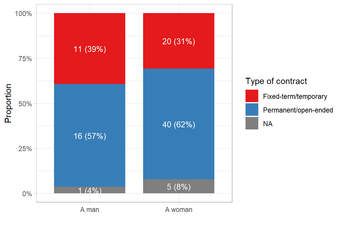
The bar chart displays the distribution of contract types by gender, showing the proportion of individuals with fixed-term and permanent contracts. Among men, 39% hold fixed-term contracts and 57% have permanent contracts. Among women, 31% are employed on a fixed-term basis, while 62% hold permanent contracts. Although the difference is moderate, the visual comparison suggests a higher proportion of fixed-term contracts among men relative to women. These figures indicate a potential association between gender and type of employment contract, which warrants further statistical analysis to determine whether the observed variation is statistically significant.
Again, we will first clean the database and apply association tests for categorical variables.
df.sub.02 <- df.geam02 |>
  filter(!is.na(WCJC011) & !is.na(SDEM004.bin)) |>
  transmute(
    TypeContract = fct_drop(WCJC011),
    Gender = fct_drop(SDEM004.bin)
)# custom function to calculate different test statistics
statsnote <- crosstab_stats(df.sub.02, "Gender", "TypeContract")
# create the contingency table
df.sub.02 |>
tbl_cross(
row = Gender,
col = TypeContract,
percent = c("row"),
) |>
bold_labels() |>
modify_footnote_header(
footnote = statsnote[[1]],
columns = last_col(),
replace=F
)
Are you on a permanent/open-ended or fixed-term/temporary contract?
|
Total1 | ||
|---|---|---|---|
| Fixed-term/temporary | Permanent/open-ended | ||
| Are you | |||
| A man | 11 (41%) | 16 (59%) | 27 (100%) |
| A woman | 20 (33%) | 40 (67%) | 60 (100%) |
| Total | 31 (36%) | 56 (64%) | 87 (100%) |
| 1 Chi-squared = 0.181 | p-value = 0.67 | df = 1 | Cramér’s V = 0.072 | Fisher’s p = 0.629 | |||
A Chi-squared test was conducted to examine whether a significant association exists between gender and contract type. The results indicate no statistically significant relationship between these variables, χ²= 0.181, p = 0.67. Furthermore, the Cramér’s V value (0.072) suggests no association, and Fisher’s exact test (p = 0.629) confirms the lack of statistical significance.
These findings imply that contract type does not significantly differ by gender within this sample.
In addition to categotrical variables, the GEAM questionnaire contains a series of continuous variables, such as age (SDEM001) or salary (WCJC005). In addition, certain questions use several sub-items which are rated by respondents on a scale of agreement or frequency. Reponses are then averaged across these items which produces a numeric score. Detecting significant differences between two (or more groups) of respondents (e.g. by gender, job position) and a numeric response variable requires different statistical techniques (student t, ANOVA), introduced in what follows.
Flexible working arrangements are key to fostering an inclusive and supportive work environment, enabling employees to balance professional and personal responsibilities. We will analyse responses to question WCWI005, which assesses employees’ awareness and use of various flexible working arrangements, including:
WCWI005.SQ001)WCWI005.SQ002)WCWI005.SQ003)WCWI005.SQ004)Note that WCWI005 is specific to the GEAM version 2. Flexible work arrangements have been revised in GEAM version 3. For an overview of the updated variables see the introduction Chapter 8.
Responses follow the response scale below.
levels(df.geam01$WCWI005.SQ001.)
#> [1] "I do not know if this is available"
#> [2] "I know that this is not available"
#> [3] "I know that this is available but I have not used it "
#> [4] "I know that this is available and I have used it"
Higher numerical values indicate greater availability and awareness of these flexible work options.
To perform the analysis, we will treat these variables as interval variables, which allows us to calculate the mean of these four items for each respondent or observation.
df.geam01 <- df.geam01 |>
  mutate(across(starts_with("WCWI005.SQ"), as.numeric),
         FlexMean = rowMeans(across(starts_with("WCWI005.SQ")), na.rm = TRUE))
The following table presents descriptive statistics for the mean flexibility score, disaggregated by gender.
df.geam01 |>
  filter(!is.na(SDEM004.bin)) |>
  group_by(SDEM004.bin) |>
  summarize(
    N = n(),
    Mean_Flex = round(mean(FlexMean, na.rm = TRUE),2),
    SD_Flex = round(sd(FlexMean, na.rm = TRUE),2),
    Median_Flex = median(FlexMean, na.rm = TRUE),
    IQR_Flex = IQR(FlexMean, na.rm = TRUE),
    .groups = "drop"
)| SDEM004.bin | N | Mean_Flex | SD_Flex | Median_Flex | IQR_Flex |
|---|---|---|---|---|---|
| A man | 87 | 3.30 | 0.52 | 3.25 | 0.75 |
| A woman | 130 | 3.17 | 0.73 | 3.25 | 0.75 |
The average score for men was 3.30 (SD = 0.52), compared to 3.17 (SD = 0.73) for women. Although the mean score was slightly higher for men, both groups shared the same median value (3.25) and interquartile range (0.75), suggesting a similar central tendency and spread in the middle 50% of responses. The standard deviation was notably higher among women, indicating greater variability in their responses. These results provide initial evidence of a modest difference in perceived workplace flexibility by gender, which warrants further statistical testing to assess its significance.
We can also demonstrate potential gender differences with a box plot. The box plot illustrates the distribution of Flexible Work scores across gender groups.
Each box represents the interquartile range (IQR), with the black horizontal line inside indicating the median value. The whiskers extend to approximately 1.5 times the IQR, and any data points beyond this range are shown as outliers.
cpal <- RColorBrewer::brewer.pal(3, "Set1")

df.sub.01|>
  ggplot(aes(x = SDEM004.bin, y = FlexMean, fill = SDEM004.bin)) +
    geom_boxplot(width = 0.5) +
    scale_fill_manual(values = cpal) +
    scale_y_continuous(limits = c(1, 4), breaks = 1:4) +
    labs(x = "", y = "Mean Flexibility Score", fill = "Gender") +
    theme_light()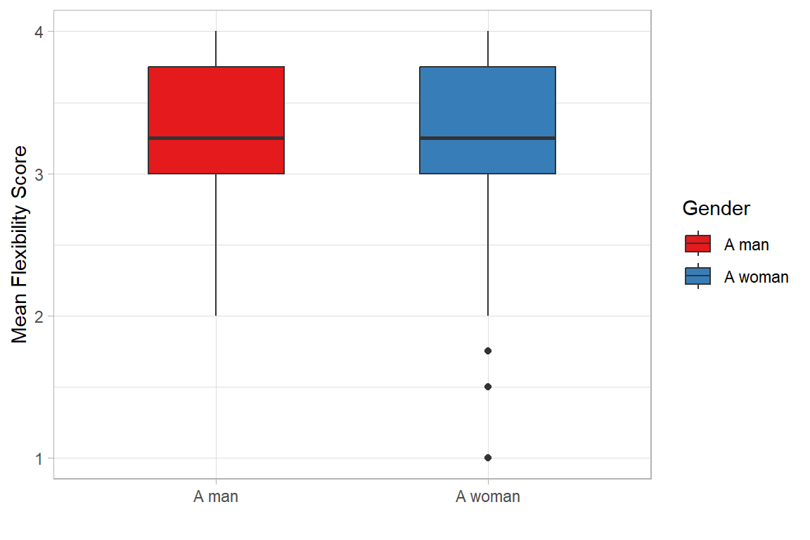
The boxplot indicates no major differences in the perception of flexible work between men and women, as their medians and interquartile ranges are quite similar.
To formally determine whether or not there are statistically significant differences, parametric tests (t-tests) or nonparametric tests (Mann-Whitney U test) will be used depending on the characteristics of the data.
Before computing the tests, we need to perform some preliminary tests to check if the assumptions are met.
The independent samples t-test assumes: 1. independence of observations, meaning that the data from one participant do not influence another; 2. normality of the dependent variable within each group, which can be assessed using the Shapiro–Wilk test or visual inspection; and 3. homogeneity of variances between groups, typically tested with Levene’s test. If normality or equal variances are violated, alternative approaches such as Welch’s t-test or non-parametric methods like the Mann–Whitney U test may be more appropriate.
df.sub.01 |>
  filter(SDEM004.bin %in% c("A woman", "A man")) |>
  group_by(SDEM004.bin) |>
  summarise(
    W = shapiro.test(FlexMean)$statistic,
    p_value = shapiro.test(FlexMean)$p.value
  ) |>
rename(Gender = SDEM004.bin)| Gender | W | p_value |
|---|---|---|
| A man | 0.9300363 | 0.000244 |
| A woman | 0.8846298 | 0.000000 |
Shapiro–Wilk tests indicated significant deviations from normality (p < 0.05).
car::leveneTest(FlexMean ~ SDEM004.bin, data = df.sub.01)| Df | F value | Pr(>F) | |
|---|---|---|---|
| group | 1 | 1.98353 | 0.1605639 |
| 201 | NA | NA |
The Levene’s test is not significant (p > 0.05). Therefore, we can assume the homogeneity of variances in the different groups.
Now, we calculate the t test or Mann-Whitney U test depending on the nature of our data.
Although the Shapiro–Wilk test indicated significant deviations from normality, the sample size in each group was sufficiently large (n > 30), allowing the application of the independent samples t-test based on the Central Limit Theorem. Furthermore, the assumption of homogeneity of variances was met.
t.test(FlexMean ~ SDEM004.bin, data = df.sub.01, var.equal = TRUE)
#>
#>  Two Sample t-test
#>
#> data:  FlexMean by SDEM004.bin
#> t = 1.3405, df = 201, p-value = 0.1816
#> alternative hypothesis: true difference in means between group A man and group A woman is not equal to 0
#> 95 percent confidence interval:
#>  -0.0591585  0.3104015
#> sample estimates:
#>   mean in group A man mean in group A woman
#> 3.295732 3.170110The independent samples t-test examined whether mean flexibility scores differed significantly by gender. The results indicated that the difference in mean scores between men (3.30) and women (3.17) was not statistically significant [t(201) = 1.34, p = 0.182]. The 95% confidence interval for the difference in means ranged from –0.06 to 0.31, suggesting that the true difference could plausibly be zero. These findings indicate that, while men reported slightly higher average flexibility scores, the observed difference is not sufficient to conclude a statistically significant gender gap in workplace flexibility within this dataset.
Job satisfaction is a critical indicator of employee well-being and organisational health. It reflects how individuals perceive their working conditions and can influence productivity, retention, and overall engagement. Exploring gender differences in job satisfaction can help identify whether workplace experiences and perceptions vary across genders, potentially revealing underlying inequalities.
Now, we will examine responses to the question EWCS88JobSatisfact1
| Code | Question | Responses |
|---|---|---|
| EWCS88JobSatisfact1 | On the whole how satisfied are you with the working conditions in your main paid job? | [1] Very satisfied [2] Satisfied [3] Somewhat satisfied [4] Not at all satisfied [5] Don’t know/no opinion |
To enable the use of parametric statistical techniques, a new numerical variable will be created to represent job satisfaction. The original categorical variable, which includes four ordered levels of satisfaction and an additional non-substantive response (“Don’t know/No opinion”), will be inverted so that higher values correspond to higher levels of satisfaction.
In addition, each response will then be recoded into a numerical score ranging from 1 (lowest satisfaction) to 4 (highest satisfaction). Uninformative responses will be excluded by assigning them a missing value (NA). The resulting variable will serve as a continuous measure of job satisfaction for subsequent statistical analyses.
df.geam03 <- df.geam03 |>
  mutate(JobSF.rev   = fct_rev(EWCS88JobSatisfact1), # reverse factor
         JobSF.score = if_else(JobSF.rev == "Don't know/no opinion",
                             NA,
as.numeric(JobSF.rev)-1) ) Now, we will investigate whether perceived job satisfaction varies as a function of gender, educational attainment, and the interaction between these two factors.
Given the relevance of both gender and education in shaping workplace experiences, a two-way analysis of variance (ANOVA) will be apply to explore potential differences in job satisfaction scores across these dimensions. This approach not only assesses the individual (main) effects of gender and education on satisfaction levels, but also examines whether the effect of education on job satisfaction differs between men and women. Identifying such interaction effects is essential for understanding how intersecting social characteristics influence perceptions of work-related well-being.
To facilitate the analysis of interaction effects and enhance comparability, the original educational attainment variable (SDEM016) will be recoded into three broader categories following the example of Listing 2.7 in Section 2.1.10. The existing answer options for SDEM016 are the following:
levels(df.geam03$SDEM016)
#>  [1] "No formal education "
#>  [2] "Primary school / elementary school"
#>  [3] "Prefer not to say"
#>  [4] "Secondary school / high school"
#>  [5] "College diploma or degree"
#>  [6] "Technical school"
#>  [7] "University - Baccalaureate / Bachelor's"
#>  [8] "University - Master's"
#>  [9] ""
#> [10] "University - Doctorate"
#> [11] "University - Postdoctorate"
#> [12] "Other"
Respondents reporting no formal education, primary, or lower secondary qualifications will be categorised as ‘Low’. Those indicating technical education, a college diploma, or a bachelor’s degree will be classified as ‘Medium’. Individuals with postgraduate education, including master’s, doctoral, or postdoctoral degrees will be assigned to the ‘High’ category. Responses such as “Prefer not to say” or “Other” will be treated as missing values and excluded from the analysis. This recoding will support a more robust and interpretable assessment of educational level as a factor in the subsequent two-way ANOVA.
df.geam03 <- df.geam03 |>
  mutate(
    educ.level = case_when(
      SDEM016 %in% c(
        "No formal education ",
        "Primary school / elementary school",
        "Secondary school / high school"
      ) ~ "Low",

      SDEM016 %in% c(
        "College diploma or degree",
        "Technical school",
        "University - Baccalaureate / Bachelor's"
      ) ~ "Medium",

      SDEM016 %in% c(
        "University - Master's",
        "University - Doctorate",
        "University - Postdoctorate"
      ) ~ "High",

      SDEM016 %in% c(
        "Prefer not to say",
        "Other",
        ""
      ) ~ NA_character_
    ),

    educ.level = factor(educ.level, levels = c("Low", "Medium", "High"))
)To ensure the validity of the statistical analysis, a clean subset of the data was created by removing any observations with missing values in the key variables of interest: job satisfaction score, gender, and educational level. This filtering step guarantees that the subsequent model includes only complete cases and avoids bias due to incomplete responses. The resulting dataset retains only the relevant variables and is used as the analytical base for the two-way ANOVA.
df.sub.03 <- df.geam03 |>
  filter(
    !is.na(JobSF.score),
    !is.na(SDEM004.bin),
    !is.na(educ.level)
  ) |>
  transmute(
    JobSF.score,
    Gender = fct_drop(SDEM004.bin),
    educ.level
  )
Then, we will calculate summary statistics (n, mean, standard deviation) by groups (gender and educational level).
df.sub.03 |>
  group_by(Gender, educ.level) |>
  summarize(
    N = n(),
    Mean_Flex = round(mean(JobSF.score, na.rm = TRUE),2),
    SD_Flex = round(sd(JobSF.score, na.rm = TRUE),2),
    Median_Flex = median(JobSF.score, na.rm = TRUE),
    IQR_Flex = IQR(JobSF.score, na.rm = TRUE),
    .groups = "drop"
)| Gender | educ.level | N | Mean_Flex | SD_Flex | Median_Flex | IQR_Flex |
|---|---|---|---|---|---|---|
| A man | Low | 8 | 2.00 | 1.07 | 2 | 1.25 |
| A man | Medium | 90 | 2.20 | 0.80 | 2 | 1.00 |
| A man | High | 29 | 2.14 | 0.83 | 2 | 1.00 |
| A woman | Low | 25 | 2.36 | 0.76 | 2 | 1.00 |
| A woman | Medium | 219 | 2.11 | 0.73 | 2 | 0.00 |
| A woman | High | 74 | 2.27 | 0.80 | 2 | 1.00 |
Among men, mean satisfaction scores are relatively consistent across education levels, ranging from 2.00 in the low education group to 2.20 in the medium group, with a slightly lower mean observed among those with higher education (2.14). In contrast, women with low education levels reported the highest average score (2.36), while those with medium education had the lowest (2.11).
Now, a boxplot will illustrate the distribution of job satisfaction scores by gender, with education level represented by colour.
cpal <- RColorBrewer::brewer.pal(3, "Set1")

df.sub.03 |>
  ggplot(aes(x=Gender, y = JobSF.score, fill=educ.level)) +
  geom_boxplot(width=.8) +
  scale_fill_manual(values=cpal) +
  scale_y_continuous(limits = c(0.5, 4.5)) +
  labs(x="", y="Mean job satisfaction", fill="Year") +
  theme_light()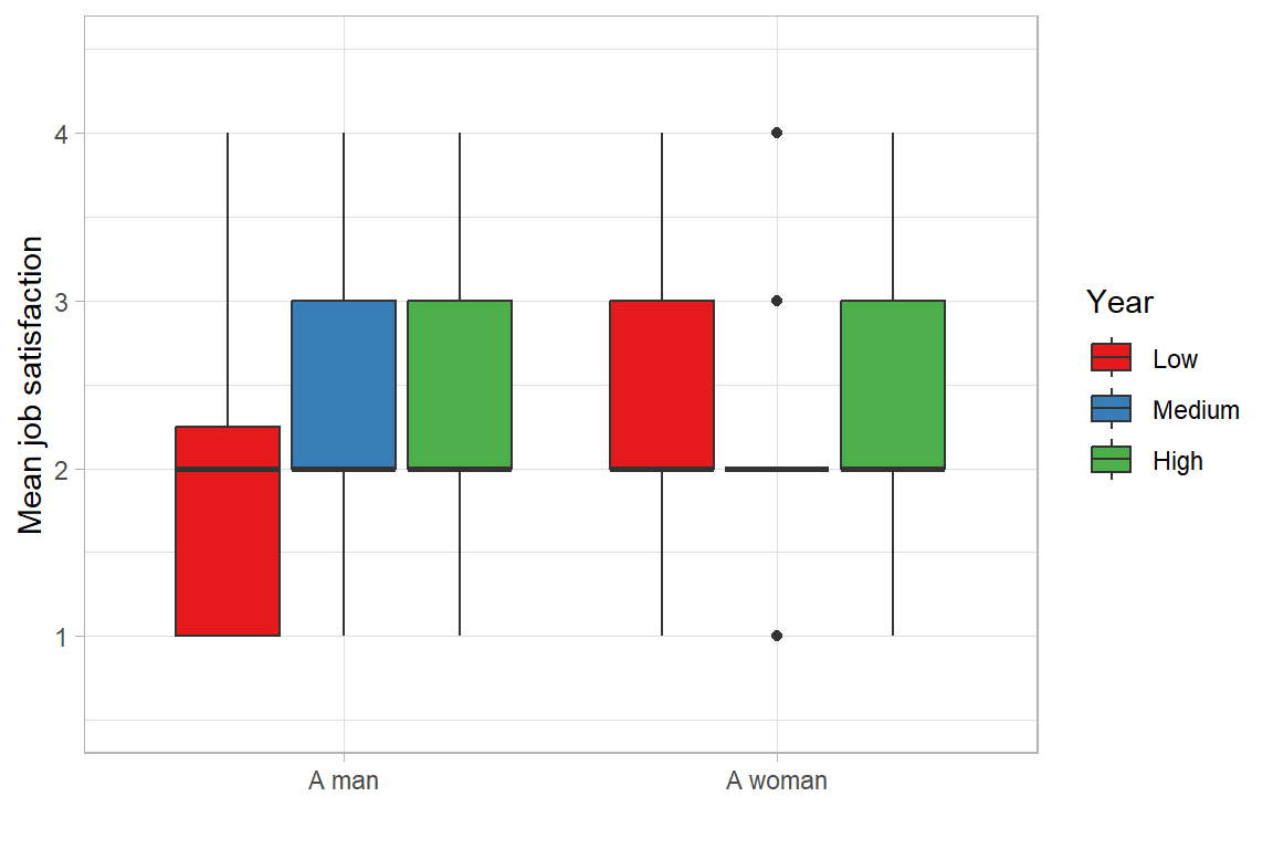
The boxplot displays job satisfaction scores by gender and education level. These descriptive patterns point to subtle differences in satisfaction across gender–education intersections, which will be further examined through inferential analysis.
Prior to apply the two-way analysis of variance (ANOVA), assumptions regarding normality and homogeneity of variances will be evaluated to ensure the suitability of the parametric approach.
# Build the linear model
model  <- lm(JobSF.score ~ Gender * educ.level,
             data = df.sub.03)

# Create a QQ plot of residuals
ggqqplot(residuals(model))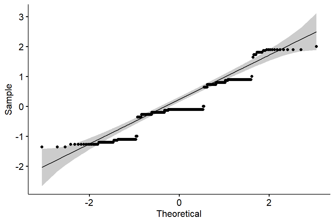
# Check normality assumption by groups
df.sub.03 %>%
group_by(Gender, educ.level) %>%
shapiro_test(JobSF.score)| Gender | educ.level | variable | statistic | p |
|---|---|---|---|---|
| A man | Low | JobSF.score | 0.8599491 | 0.1199348 |
| A man | Medium | JobSF.score | 0.8534021 | 0.0000001 |
| A man | High | JobSF.score | 0.8511970 | 0.0008049 |
| A woman | Low | JobSF.score | 0.8525910 | 0.0019732 |
| A woman | Medium | JobSF.score | 0.8044540 | 0.0000000 |
| A woman | High | JobSF.score | 0.8549790 | 0.0000005 |
The assumption of normality was assessed through both statistical testing and visual inspection of the model residuals. The Shapiro–Wilk test indicated a statistically significant deviation from normality, likely driven by the discrete nature of the dependent variable and the high frequency of tied values. However, the Q–Q plot of the residuals showed only minor departures from the theoretical line, suggesting no severe violation.
Moreover, the sample sizes within most groups—particularly those with medium and high levels of education—were sufficiently large to invoke the Central Limit Theorem. Therefore, despite the significant result from the normality test, the assumption is considered reasonably met, and the ANOVA may proceed with caution.
car::leveneTest(JobSF.score ~ Gender * educ.level, data=df.sub.03)| Df | F value | Pr(>F) | |
|---|---|---|---|
| group | 5 | 1.585501 | 0.1627715 |
| 439 | NA | NA |
The Levene’s test is not significant (p > 0.05). Therefore, we can assume the homogeneity of variances in the different groups.
anova_model <- aov(JobSF.score ~ Gender * educ.level, data = df.sub.03)
summary(anova_model)
#>                    Df Sum Sq Mean Sq F value Pr(>F)
#> Gender              1   0.01  0.0086   0.014  0.905
#> educ.level          2   1.19  0.5933   0.999  0.369
#> Gender:educ.level   2   1.71  0.8560   1.441  0.238
#> Residuals 439 260.79 0.5940A two-way analysis of variance was conducted to examine the effects of gender and education level on job satisfaction scores, as well as their interaction. The results indicated that there were no statistically significant main effects for gender (F(1, 439) = 0.014, p = 0.905) or education level (F(2, 439) = 0.999, p = 0.369). Furthermore, the interaction between gender and education was not significant (F(2, 439) = 1.441, p = 0.238). These findings suggest that, within this sample, job satisfaction does not differ meaningfully by gender, education level, or their combination.
Conclusion: Although prior research has often pointed to the potential influence of gender and educational attainment on perceptions of job satisfaction, the present analysis did not reveal statistically significant differences across these dimensions. Neither gender nor education level appeared to have a measurable impact on satisfaction scores, nor was there evidence of an interaction between the two. These findings may reflect a genuinely uniform experience of satisfaction across groups in this particular organisational context, or they may be shaped by the limited range and distribution of the satisfaction scale. Further research using alternative measures or larger samples may help clarify whether these results are sample-specific or indicative of broader patterns.